Download
1 / 16
160 likes | 267 Views
Sorting in Linear Time. 7.1 Lower bounds for sorting. 本節探討排序所耗用的時間複雜度下限。 任何一個以比較為基礎排序的演算法,排序 n 個元素時至少耗用 Ω ( n log n ) 次比較。 是以時間複雜度至少為 Ω ( n log n ) 。 但不使用比較為基礎 的排序演算法,在某些情形下可在 O(n) 的時間內執行完畢。. Decision-Tree Model. 一個以比較為基礎的排序演算法可以按照比較的順序建出一個 Decision-Tree 。 每一個從 Root 到 Leaf 的路徑都代表一種排序的結果。

E N D
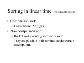
7.1 Lower bounds for sorting • 本節探討排序所耗用的時間複雜度下限。 • 任何一個以比較為基礎排序的演算法,排序n個元素時至少耗用Ω(nlogn)次比較。 是以時間複雜度至少為Ω(nlogn)。 • 但不使用比較為基礎 的排序演算法,在某些情形下可在O(n)的時間內執行完畢。 Sorting in Linear Time
Decision-Tree Model • 一個以比較為基礎的排序演算法可以按照比較的順序建出一個Decision-Tree。 • 每一個從Root到Leaf的路徑都代表一種排序的結果。 • 任何一個以比較為基礎排序n個元素的演算法,所對應的Decision-Tree高度至少有Ω(nlogn)。 Sorting in Linear Time
Decision-Tree Model Eg. (a1 a2 a3) (9 2 6) a1:a2 > a1:a3 a2:a3 > > <1,2,3> a1:a3 <2,1,3> a2:a3 > > <1,3,2> <3,1,2> <2,3,1> <3,2,1> Sorting in Linear Time
Decision-Tree Model • 證明:因為可能有n!種可能的排序結果,故對應的Decision tree至少有n!個leaf nodes。而高度為h的二元樹最多有2h個leaf nodes。因此h log2(n!) Θ(nlogn)。(後者由Stirling’s approximation得證:n!>(n/e)n) • Heapsort與Mergesort是asymptotically optimal之比較排序法。 Sorting in Linear Time
7.2 Counting Sort • Counting Sort (記數排序法) 不需要藉由比較來做排序。 • 必須依賴一些對於待排序集合中元素性質的假設。(如:所有待排序元素均為整數,介於1到k之間) • 時間複雜度:O(n+k) • 主要的關鍵在於,統計1到k之間每個數值出現過幾次,然後想辦法將排序好的數列輸出。 Sorting in Linear Time
Input: A[1..n], where A[j]∈{1,2,…,k} Output:B[1..n], sorted CountingSort(A,B,k) { for i = 0 to k do C[i]0 for j = 1 to length[A] do C[A[j]]C[A[j]]+1 for i = 1 to k do C[i]C[i]+C[i-1] for j = length[A] downto 1 do B[C[A[j]]]A[j] C[A[j]]C[A[j]]-1 } Sorting in Linear Time
k=6 1 2 3 4 5 6 7 8 A: 3 6 4 1 3 4 1 4 1 2 3 4 5 6 2nd loop C: 2 0 2 3 0 1 1 2 3 4 5 6 3rd loop 2 2 4 7 7 8 Sorting in Linear Time
4th loop 1 2 3 4 5 6 7 8 1 2 3 4 5 6 1st iteration B: C: 4 2 2 4 6 7 8 1 2 3 4 5 6 7 8 1 2 3 4 5 6 2nd iteration B: C: 1 4 1 2 4 6 7 8 1 2 3 4 5 6 7 8 1 2 3 4 5 6 3rd iteration B: C: 1 4 4 1 2 4 5 7 8 …… 1 2 3 4 5 6 7 8 1 2 3 4 5 6 8th iteration B: C: 1 1 3 3 4 4 4 6 0 2 2 4 7 7 Sorting in Linear Time
7.3 Radix Sort • Radix Sort(基數排序法)無需利用元素間的比較排序。 • 必須依賴一些對於待排序集合中元素性質的假設。(所有待排序元素均為整數,至多d位) Sorting in Linear Time
Radix Sort • 關鍵想法:利用記數排序法由低位數排到高位數。 329 457 657 839 436 720 355 720 355 436 457 657 329 839 720 329 436 839 355 457 657 329 355 436 457 657 720 839 最後排百位數 先排個位數 再排十位數 Sorting in Linear Time
Radix-Sort(A,d) { for i = 1 to d do use stable sort to sort A on digit i } • 此處使用的stable sort如果使用Counting Sort則每個Iteration只需花Θ(n+10)的時間。 • 因此總共花費O(d(n+10))的時間。 • 如果d是常數,則Radix Sort為一個可以在Linear time完成的排序演算法。 Sorting in Linear Time
7.4 Bucket Sort • 當元素均勻分布在某個區間時,Bucket sort平均能在O(n)的時間完成排序。 • 假定要排序n個元素A[1..n]均是介於[0,1]之間的數值。 • 準備n個籃子(bucket),B[1..n],將元素x依照x所在的區間放進對應的籃子:即第 個籃子 。 Sorting in Linear Time
Bucket Sort • 元素放進籃子時,使用Linked list來儲存,並利用插入排序法排序。 • 只要依序將Lined list串接起來,即得到已排序的n個元素。 Sorting in Linear Time
A B 1 .76 1 .05 .07 2 .07 2 3 .36 3 .22 .25 .29 4 .29 4 .36 5 .74 5 6 6 .95 7 .22 7 .66 8 .05 8 .74 .76 9 .25 9 10 .66 10 .95 紅色虛線串起的即是最後排序好的List Sorting in Linear Time
時間複雜度分析 • 假定分到第i個籃子的元素個數是ni。 • 最差情形:T(n) =O(n) + =O(n2). • 平均情形:T(n) = O(n) + = O(n) + = O(n) • 的証明請參考課本 Sorting in Linear Time