Download
1 / 33
330 likes | 442 Views
30 September 2002. ECEE 302: Electronic Devices. In Preparation for Next Monday. Lecture 2. Physical Foundations of Solid State Physics. Outline. Characteristics of Quantum Mechanics Black Body Radiation Photoelectric Effect Bohr’s Atom and Spectral Lines de Broglie relations

E N D
30 September 2002 ECEE 302: Electronic Devices In Preparation for Next Monday Lecture 2. Physical Foundations of Solid State Physics
Outline • Characteristics of Quantum Mechanics • Black Body Radiation • Photoelectric Effect • Bohr’s Atom and Spectral Lines • de Broglie relations • Wave Mechanics • Probability • Schrodinger Equation • Uncertainty Relations • Applications of Wave Mechanics • Infinite Well • Finite Barrier (Tunneling) • Hydrogen Atom • Periodic Table • Pauli Exclusion Principle • Minimum Energy • Bohr’s Aufbauprinzip (Building-Up Principle) • Atomic Structure
What is Quantum Mechanics? • Classical Mechanics • Newton’s Three Laws • applies to particles (localized masses) or mass distributions • Well defined deterministic trajectories • Initial Conditions and Equations of Motion determine particle behavior for all time • Classical Optics • Light is wave (non-localized, spread over region) • Interference and Diffraction effects are seen • Quantum Mechanics • Laws based on Geometrical Optics (short wave-length region) • Describes system behavior in terms of “Wave Function” • “square of wave function” provides probabilistic information about state of system • Evolution of Wave Function in Time is deterministic • An observation based on the wave function • possible outcomes of observation • probability of each outcome
Black Body Radiation • Black Body is perfect absorber (and re-radiator) • Based on classical mechanics, the black body should have infinite energy • Planck found an empirical formula to fit Black Body experimental curve • To derive this formula from first principles he had to assume light energy (electromagnetic energy) was not spread out in space but came in small packages or bundles (quanta - german word for “dose”). E=hn Classical Equi-partition of Energy Model Thermal (Black Body) Energy Frequency
Photo-Electric Effect • When light of frequency n is incident on a metal, electrons are emitted from the metal • Emission is instantaneous • kinetic energy of the emitted electrons are dependent on the frequency of the light (n) • Einstein (1905) used Planck’s idea of bundle of light to explain this effect • (1/2) mv2=hn-F • Einstein called this particle of light a “photon” • Einstein had shown that Planck’s hypothesis could be interpreted as showing that waves can exhibit particle like properties F=Work Function
The Crisis in Atomic Theory • Ernst Rutherford determined the atom has a small positvely charged, solid nucleus which is surrounded by a swarm of negatively charged electrons • Classical Electrodynamics predicted that an accelerating particle (such as an electron moving around the nucleus of an atom) should radiate continuously, reduce its radius until it spirals into the nucleus • Observation shows us that • Atoms are stable • Radiation from atoms is with discrete spectral lines that follow a geometric series • Niels Bohr resolved these issues with a new atomic model based on the work of Einstein and Planck
The Atom of Neils Bohr • Postulates • Atoms are stable • Electrons can exist in well defined orbits around a nucleus (Atomic State) • Electrons do not radiate when in the orbit (Contrary to Classical Electromagnetism) • Discrete Spectral lines • Atoms radiate (emit a photon) or absorb energy (absorb a photon) when an electron makes a transition from one fixed orbit (initial state) to another orbit (final state) • The frequency of the light emitted or absorbed is given by Planck’s formula n=DE/h • The discrete orbits are determined by “quantization” of the orbital angular momentum. This is determined by the relation mvrn=nh • This theory successfully reproduced the spectral line pattern seen in H, He+, and Li++, single electron atoms
Bohr’s Atom (1 of 3) e Ze
The atom of Bohr Kneels(“The Strange Story of the Quantum” - Banesh Hoffman) • Bohr’s Theory failed to predict the spectral behavior of more complex atoms with two or more electrons • Spectral line splitings (fine structure) was not predicted by Bohr’s Theory • The anomalous Zeeman effect (splitting of spectral lines in Magnetic Fields) was also not predicted successfully • This required a more fundamental theory
Davision-Germer Experiment and the de Broglie Hypothesis • In 19XX Davision and Germer of the Bell Telephone Laboratories showed that high energy electrons could be diffracted by crystals • Particles had shown characteristics of waves • Louis de Broglie characterized the wave nature of particles by the expression l=h/p • localized particle properties: Energy & Momentum • non-local wave properties: frequency & wavelength Characteristicsmassenergymomentum Wave (light) 0 E=hn p=hk=h/l=E/c Particles (~electron) m E=hn p=hk=h/l=(2mE)1/2
Wave Mechanics (1 of 2) • Schrodinger used classical geometrical optics to formulate a new mechanics he called wave mechanics
Physical Interpretation of y • Schrodinger initially believed that Y was a guiding wave • Max Born introduced a probability interpretation for Y The change in probability within a volume V is due to the “flow” of propability across the bounding surface A
Solutions of the Schrodinger Equation • The Schrodinger equation is a second order differential equation • It can be split into the product of a time solution and a spatial solution by the method of separation of variables • Q(r,t)=A( r) B(t) • Show equations for t and for r • The spatial equation is called a sturm-louisville equation. Solutions exist only for certain values of the separation constant. These are called eigen (proper) solutions and eigen (proper) values • These possible solutions are called quantum levels and the specific values are called quantum values (or quantum numbers) • The corresponding functions are called quantum state functions
Boundary Conditions • Solutions must obey the following conditions called boundary conditions • Q must be bounded (finite) everywhere • At boundaries between multiple solutions the magnitude and the derivative of the solutions must be continuous
Normalization of the Wave Function • Since Q is a probability amplitude and QQ* is a probability we must have • integral of QQ* over all space = 1 • This is called normalization of the wave function • Examples • Particle in a box • Hydrogen Equation
Applications • Potential Well - (Stationary States) • Potential Barrier - (Tunneling) • Hydrogen Atom (quantum numbers) • Electron Spin • Hydrogen Molecule • Bonds • Ionic Bond • Valence Bond
Potential Well (in 1-dimension) and Bound States • Schrodinger Equation • Boundary Conditions • Solutions • Quantization of Energy Levels • Uncertainty Principle
Potential Barrier in 1 dimension (Tunneling) • Schrodinger Equation • Boundary Conditions • Solution • Uncertainty Principle
Hydrogen Atom • Schrodinger Equation in 3 dimensions • Schrodinger Equation in spherical coordinates • Separation of Variable for r, q, h • Solution for h = magnetic quantum number • Legendre polynomials for q = angular momentum quantum number • Legarre polynomials for r = principle (orbital) quantum number • Electron spin s=+/- 1/2 • Designation of a quantum state n,l,m,s
Uncertainty Principle • Introduced by Werner Heisenberg • Statement of Uncertainty Relations • Uncertainty in position x uncertainty in momentum > h • Uncertainty in energy x uncertainty in time > h
Hydrogen Molecule • Schrodinger Equation • Solution • Interpretation • Electron Spin
Ionic Bond • Ionic Bonding • exchange of an electron between two atoms so each acheives a closed shell • result is a positive (electron donor) and negative (electron acceptor) ion • ions attract forming a bond • Examples: NaCl, KCl, KFl, NaFl
Valance Bond • Valance Bond: Bonding due to two atoms of complementary valance combining chemically • Valance Band 4 (and 4): C, Si, Ge, SiC • Valance Band 3 and 5: GaAs, InP, • Valance Band 2 and 6: CdS, CdTe • Examples • Face Centered Cubic: Diamond (C), Silicon (Si)
Periodic Table of Elements • History • Developed by Medelaev in 1850 based on chemical properties of atoms • Understood initially in terms of chemical affinities (Valence) • Quantum Mechanics provides the Physical Theory of Valence • Atoms are arranged in 8 basic columns related to the valence of each atom • Transition elements build up their electronic structure • Periodic Table can be understood in terms of two principles • Pauli Exclusion Principal • Minimum Energy Principal
Pauli Exclusion Principle • No two electrons can be in the same quantum state at the same time • Fundamental in understanding the structure of the periodic table
Bohr’s Building up (Aufbauprinzip) Principle • Determines the basic structure of atoms • Based on the Pauli Exclusion Principle • Minimum Energy Principal
Minimum Energy Criteria • Over-arching principle is minimum energy • explains electronic structure of rare earth elements
Atomic Structure • Quantum Numbers • n-principal quantum number signifies the electron orbit • l-orbital quantum number signifies the angular momentum in orbit n (l=0,1,2,…,n-1) • m - magnetic quantum number signifies the projection of the angular momentum quantum number on a specific axis (z), (m=-l,-(l-1), -(l-2), …,-1,0,1,…,(l-1),l) • s - electron spin signifies and internal state of the electron (s=+1/2, -1/2) • Atom is described by the set of quantum numbers that describe each electron state • Hydrogen = 1s1 X Potassium 1s2,1p6,2s1 • Helium = 1s2 Carbon 1s2, 1p4 1s2,1p6,2s2 • Lithium = 1s2,11p1 Nitrogen • Boron = 1s2, 1p2 Neon 1s2, 1p6