Download

1 / 68
680 likes | 935 Views
Inside Internet Routers. CS 3035/GZ01: Networked Systems Kyle Jamieson Department of Computer Science University College London. Today: Inside Internet routers. Longest-prefix lookup for IP forwarding T he Luleå algorithm Router architecture. Cisco CRS-1 Carrier Routing System.

E N D
Inside Internet Routers CS 3035/GZ01: Networked Systems Kyle Jamieson Department of Computer Science University College London
Today: Inside Internet routers • Longest-prefix lookup for IP forwarding • The Luleå algorithm • Router architecture Cisco CRS-1 Carrier Routing System
The IP forwarding problem • Core Internet links have extremely fast line speeds: • SONET optical fiber links • OC-48 @ 2.4 Gbits/s: backbones of secondary ISPs • OC-192 @ 10 Gbits/s: widespread in the core • OC-768 @ 40 Gbits/s: found in many core links • Internet routers must handle minimum-sized packets (40−64 bytes) at the line speed of the link • Minimum-sized packets are the hardest case for IP lookup • They require the most lookups per second • At 10 Gbits/s, have 32−51 nsto decide for each packet • Compare: DRAM latency ≈ 50 ns; SRAM latency ≈ 5 ns
The IP forwarding problem (2) • Given an incoming packet with IP destination D, choose an output port for the packet by longest prefix match rule • Then we will configure the switching fabric to connect the input port of the packet to the chosen output port • What kind of data structure can we use for longest prefix match?
Longest prefix match (LPM) • Given an incoming IP datagram to destination D • The forwarding tablemaps a prefix to an outgoing port: • Longest prefix match rule: Choose the forwarding table entry with the longest prefix P/x that matches Din the first xbits • Forward the IP datagram out the chosen entry’s outgoing port
Computing the longest prefixmatch (LPM) • The destination matchesforwarding table entry 192.0.0.0/4 Forwarding Table: IP Header Destination: 201.10.7.17 Destination: 201 10 7 17 1100100100001010 00000111 00010001 192 11000000 Prefix (/4):
Computing the longest prefixmatch (LPM) • No match for forwarding table entry 4.83.128.0/17 Forwarding Table: IP Header Destination: 201.10.7.17 Destination: 201 10 7 17 11001001 00001010 00000111 00010001 4 83 128 00000100 01010011 10000000 Prefix (/17):
Computing the longest prefixmatch (LPM) • The destination matchesforwarding table entry 201.10.0.0/21 Forwarding Table: IP Header Destination: 201.10.7.17 Destination: 201 10 7 17 11001001000010100000011100010001 201 10 0 110010010000101000000000 Prefix (/21):
Computing the longest prefixmatch (LPM) • The destination matchesforwarding table entry 201.10.6.0/23 Forwarding Table: IP Header Destination: 201.10.7.17 Destination: 201 10 7 17 11001001000010100000011100010001 201 10 6 110010010000101000000110 Prefix (/21):
Computing the longest prefixmatch (LPM) • Applying the longest prefix match rule, we consider only all three matching prefixes • We choose the longest, 201.10.6.0/23 Forwarding Table: IP Header Destination: 201.10.7.17
LPM: Performance • How fast does the preceding algorithm run? • Number of steps is linear in size of the forwarding table • Today, that means 200,000−250,000 entries! • And, the router may have just tens of nanoseconds before the next packet arrives • Recall, DRAM latency ≈ 50 ns; SRAM latency ≈ 5 ns • So, we need muchgreater efficiency to keep up with line speed • Better algorithms • Hardware implementations • Algorithmic problem: How do we do LPM faster than a linear scan?
First attempt: Binary tree • Store routing table prefixes, outgoing port in a binary tree • For each routing table prefix P/x: • Begin at root of a binary tree • Start from the most-significant bit of the prefix • Traverse down ith-level branch corresponding to ith most significant bit of prefix, store prefix and port at depth x Length (bits) Root 1 0 80/1 00/1 1 0 80/2 C0/2 Note convention: Hexadecimal notation
Example: 192.0.0.0/4 in the binary tree Forwarding Table: Root 1 80/1 1 C0/2 0 0xC0 11000000 C0/3 192.0.0.0/4: 0 C0/4: Port 2
Routing table lookups with the binary tree • When a packet arrives: • Walk down the tree based on the destination address • The deepestmatching node corresponds to the longest-prefix match • How much time do we need to perform an IP lookup? • Still need to keep big routing table in slow DRAM • In the worst case, scales directly with the number of bits in longest prefix, each of which involves a slow memory lookup • Back-of-the-envelope calculation: • 20-bit prefix × 50 ns DRAM latency = 1 μs (goal, ≈ 32 ns)
Luleå algorithm • Degermark et al., Small Forwarding Tables for Fast Routing Lookups (ACM SIGCOMM ‘97) • Observation: Binary treeis too large • Won’t fit in fast CPU cache memory in a software router • Memory bandwidth becomes limiting factor in a hardware router • Therefore, goal becomes: How can we minimize memory accesses and the size of data structure? • Method for compressing the binary tree • Compact 40K routing entries into 150−160 Kbytes • So we can use SRAM for the lookup, and thus perform IP lookup at Gigabit line rates!
Luleå algorithm: Binary tree • The full binary tree has a height of 32 (number of bits in IP address) • So has 232 leaves (one for each possible IP address) • Luleå stores prefixes of different lengths differently • Level 1 stores prefixes ≤ 16 bits in length • Level 2 stores prefixes 17-24 bits in length • Level 3 stores prefixes 25-32 bits in length 0 31 IP address space: 232 possible addresses
Luleå algorithm: Level 1 • Imagine a cutacross the binary tree at level 16 • Construct a length 216bit vectorthat contains information about the routing table entries at or above the cut • Bit vector stores one bit per /16 prefix • Let’s zoom in on the binary tree here: 0 Level-16 cut 31 IP address space: 232 possible addresses
Constructing the bit vector • Put a 1 in the bit vector wherever there is a routing table entry at depth ≤ 16 • If the entry is abovelevel 16, follow pointers left(i.e., 0) down to level 16 • These routing table entries are called genuine heads … … … 1 1
Constructing the bit vector • Put a 0 in the bit vector wherever a genuine head at depth < 16 containsthis /16 prefix • For example, 0000/15 contains0001/16 (they have the same next hop) • These routing table entries are called members … … … 1 0 1
Constructing the bit vector • Put a 1in the bit vector wherever there are routing entries at depth > 16, belowthe cut • These bits correspond to root heads, and are stored in Levels 2 and 3 of the data structure … … … 1 0 1 1
Bit masks • The bit vector is divided into 212 16-bit bit masks • From the figure below, notice: • The first 16 bits of the lookup IP address index the bit in the bit vector • The first 12 bits of the lookup IP address index the containing bit mask 000/12 depth 12 … 0000/16 depth 16 … Bit vector: 1 0 0 0 1 0 1 1 1 0 0 0 1 1 1 1 Bit mask
The pointer array • To compressrouting table, Luleåstores neither binary tree nor bit vector • Instead, pointer array has one entry per set bit (i.e., equal to 1) in the bit mask • For genuineheads, pointer field indexes into a next hop table • For rootheads, pointer field indexes into a table of Level 2 chunks • Given a lookup IP, how to compute the correct index into the pointer array, pix? • No simple relationship between lookup IP and pix … ‸ Pointer array type (2) pointer (14) … 1 0 0 0 1 0 1 1 1 0 0 0 1 1 1 1 pix … Genuine Next hop index Next hop index Genuine Root L2 chunk index …
Finding the pointer group: Code word array • Group the pointers associated with each bit mask together (pointer group) • The code word array stores the index in the pointer array index where each pointer group begins in its sixfield • code has 212 entries, one for each bit mask • Indexed by top 12 bits of the lookup IP six code: 000: 0 001/12 000/12 001: 9 0000/16 212 002: 14 … 1 0 0 0 1 0 1 1 1 0 0 0 1 1 1 1 1 0 0 0 0 0 0 0 1 0 1 1 1 0 0 0 Bit mask for 000/12 (nine bits set) Bit mask for 001/12 (five bits set)
Finding the pointer group: Base index array • After four bit masks, 4 × 16 = 64 bits could be set, too many to represent in six bits, so we “reset” sixto zero every fourth bit mask • The base index array basestores the index in the pointer array where groups of four bit masks begin • Indexed by the top 10 bits of the lookup IP six code: 000: 0 001: 9 002: 212 14 004/10 000/10 So, the pointer group begins at base[IP[31:22]] + code[IP[31:20]].six 003: 16 004: 0 004/12 … 000/12 (9 bits set) 001/12 (5 bits set) 002/12 (2 bits set) 003/12 (2 bits set) 004/12 (2 bits set) base: 16 bits 000: 0 001: 18 210 …
Finding the correct pointer in the pointer group • The high-order 16 bits (31−16) of the lookup IP identify a leaf at depth 16 • Recall: The first 12 of those (31−20) determine the bit mask • The last four of those (19−16, i.e.the path between depth 12 and depth 16) determine thebit within a bit mask • The maptabletells us how many pointers to skip in the pointer group to find a particular bit’s pointer • There are relatively few possible bit masks, so store all possibilities … depth 12 IP[19]: IP[18]: … IP[17]: 1 0 0 0 1 0 1 1 1 0 0 0 1 1 1 1 IP[16]: depth 16 Bit mask
Completing the binary tree • But, a problem: two different prefix trees can have the same bit vector, e.g.: … … … … … … … … … 1 0 1 1 1 0 • So, the algorithm requires that the prefix tree be complete: each node in the tree have either zeroor twochildren • Nodes with a single child get a sibling node added with duplicate next-hop information as a preliminary step
How many bit masks are possible? • Bit masks are constrained: not all 216 combinations are possible, since they are formed from a complete prefix tree • How many are there? Let’s count: • Let a(n) be the number of valid non-zero bit masks of length 2n • a(0) = 1 (one possible non-zero bit mask of length one) • a(n) = 1 + a(n − 1)2 • Either bit mask with value 1, or any combination of non-zero, half-size masks • e.g.a(1): [1 1] [1 0] • a(4) = 677 possible non-zero bit masks of length 16 • So we need 10 bits to index the 678 possibilities
Finding the correct pointer in the pointer group • tenfield of code word array stores a row index of maptablethat has offsets for the bit mask pattern at that location in the tree • Bits 19−16 of the IP address index maptable columns, to get the right (4-bit) offset in the bit mask of the bit we’re interested in • maptableentries are pre-computed, don’t depend on the routing table 0 1 2 3 4 . . . 15 IP address 0 31 maptable: 675 10 2 4 16 ten six code: maptable entry 212 0
Luleå: Summary of finding pointer index ten = code[ix].ten six = code[ix].six pix = base[bix] + six + maptable[ten][bit] pointer = pointer_array[pix]
Optimization at level 1 • When the bit mask is zero, or has a single bit set, the pointer array is holding an index into the next-hop table (i.e., a genuine head) • In these cases, store the next-hop index directly in the codeword 000/12 000/11 0 0 0 0 0 0 0 0 0 0 0 0 0 0 0 0 0 0 0 0 0 0 0 0 0 0 0 0 0 0 0 1 Bit mask Bit mask • This reduces the number of rows needed for maptable from 678 to 676
Luleå algorithm: Levels 2 and 3 • Root heads point to subtrees of height at most eight, called chunks • A chunk itself contains at most 256 heads • There are three types of chunk, depending on how many heads it contains: • Sparse: 1-8 heads, array of next hop indices of the heads within a chunk • Dense: 9-64 heads, same format as Level 1, but no base index • Very dense: 65-256 heads, same format as Level 1 Pointer array type (2) pointer (14) pix Genuine Next hop index L2 chunk index Root Genuine Next hop index …
Sprint routing table lookup time distribution(Alpha 21164 CPU) • Fastest lookups (17 cycles = 85 ns): code word directly storing next-hop index • 41 clock cycles: pointer in level 1 indexes next-hop table (genuine head) • Longer lookup times correspond to searching at levels 2 or 3 Count 500 ns worst-case lookup time on a commodity CPU 17 41 (cycle time = 5 ns)
Luleå algorithm: Summary • Current state of the art in IP router lookup • Tradeoff mutability and table construction time for speed • Adding a routing entry requires rebuilding entire table • But, routing tables don’t often change, and they argue they can sustain one table rebuild/second on their platform • Table size: 150 Kbytes for 40,000 entries, so can fit in fast SRAM on a commodity system • Utilized in hardware as well as software routers to get lookup times down to tens of nanoseconds
Today: Inside Internet routers • Longest-prefix lookup for IP forwarding • The Luleå algorithm • Router architecture • Crossbar scheduling and the iSLIP algorithm • Self-routing fabric: Banyan network Cisco CRS-1 Carrier Routing System
Router architecture • Data path: functions performed on each datagram • Forwarding decision • Switching fabric (backplane) • Output link scheduling • Control plane: functions performed relatively infrequently • Routing table information exchange with others • Configuration and management • Key design factor: Rate at which components operate (packets/sec) • If one component operates at n times rate of another, we say it has speedupof n relative to the other
Input port functionality • IP address lookup • CIDR longest-prefix match • Uses a copy of forwarding table from control processor • Check IP header, decrement TTL, recalculate checksum, prepend next-hop link-layer address • Possible queuing, depending on design R
Switching fabric • So now the input port has tagged the packet with the right output port (based on the IP lookup) • Job of switching fabric is to move the packet from an input port to the right output port • How can this be done? • Copy it into some memory location and out again • Send it over a shared hardware bus • Crossbar interconnect • Self-routing fabric
Switching via shared memory • First generation routers: traditional computers with switching under direct control of CPU • Packet copied from input port across shared bus to RAM • Packet copied from RAM across shared bus to output port • Simple design • All ports share queue memory in RAM • Speed limited by CPU: must process every packet [Image: N. McKeown]
Switching via shared bus • Datagram moves from input port memory to output port memory via a shared bus • e.g.Cisco 5600: 32 Gbit/s bus yields sufficient speed for access routers • Eliminates CPU bottleneck • Bus contention: switching speed limited by shared bus bandwidth • CPU speed still a factor [Image: N. McKeown]
Switched interconnection fabrics • Shared buses divide bandwidth among contenders • Electrical reason: speed of bus limited by # connectors • Crossbar interconnect • Up to n2 connects join ninputs to n outputs • Multiple input ports can then communicate simultaneously with multiple output ports [Image: N. McKeown]
Switching via crossbar • Datagram moves from input port memory to output port memory via the crossbar • e.g. Cisco 12000 family: 60 Gbit/s; sufficient speed for core routers • Eliminates bus bottleneck • Custom hardware forwarding engines replace general purpose CPUs • Requires algorithm to determine crossbar configuration • Requires n× output port speedup Crossbar [Image: N. McKeown]
Where does queuing occur? • Central issue in switch design; three choices: • At input ports (input queuing) • At output ports (output queuing) • Some combination of the above • n = max(# input ports, # output ports)
Output queuing • No buffering at input ports, therefore: • Multiple packets may arrive to an output port in one cycle; requires switch fabric speedup of n • Output port buffers all packets • Drawback: Output port speedup required: n
Input queuing • Input ports buffer packets • Send at most one packet per cycle to an output port
Input queuing: Head-of-line blocking • One packet per cycle sent to any output • Blue packet blocked despite the presence of available capacity at output ports and in switch fabric • Reduces throughput of the switch
Virtual output queuing • On eachinput port, place one input queue per output port • Use a crossbarswitch fabric • Input port places packet in virtual output queue (VOQ) corresponding to output port of forwarding decision • No head-of-line blocking • All ports (input and output) operate at same rate • Need to schedule fabric: choose which VOQs get service when Output ports (3)
Virtual output queuing [Image: N. McKeown]
Today: Inside Internet routers • Longest-prefix lookup for IP forwarding • The Luleå algorithm • Router architecture • Crossbar scheduling and the iSLIP algorithm • Self-routing fabric: Banyan network Cisco CRS-1 Carrier Routing System
Crossbar scheduling algorithm: goals • High throughput • Low queue occupancy in VOQs • Sustain 100% of rate R on all n inputs, n outputs • Starvation-free • Don’t allow any one virtual output queue to be unserved indefinitely • Speed of execution • Should not be the performance bottleneck in the router • Simplicity of implementation • Will likely be implemented on a special purpose chip
iSLIP algorithm: Introduction • Model problem as a bipartite graph • Input port = graph node on left • Output port = graph node on right • Edge (i, j) indicates packets in VOQ Q(i, j) at input port i • Scheduling = a bipartitematching(no two edges connected to the same node) Request graph Bipartite matching