Support Vector Machines

1. Support Vector Machines Jianping Fan Dept of Computer Science UNC-Charlotte

2. What is data classification Data Classification is approximated as data modeling!

3. What is data classification d c Data classification is approximated as data partitioning!

4. What is data classification • What is the best modeling? • What is the best partitioning? • Discriminative vs. not-discriminative

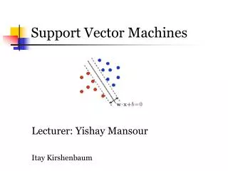
5. Which of the linear separators is optimal? Binary case

6. Best Linear Separator?

7. Best Linear Separator?

8. Best Linear Separator?

9. Best Linear Separator?

10. Find Closest Points in Convex Hulls d c

11. Plane Bisect Closest Points wT x + b =-1 wT x + b =0 d c wT x + b =1

12. Linear Discriminant Function • Binary classification can be viewed as the task of separating classes in feature space: wTx + b = 0 wTx + b > 0 wTx + b < 0 f(x) = sign(wTx + b)

13. denotes +1 denotes -1 Linear Discriminant Function x2 • How would you classify these points using a linear discriminant function in order to minimize the error rate? • Infinite number of answers! x1

14. denotes +1 denotes -1 Linear Discriminant Function x2 • How would you classify these points using a linear discriminant function in order to minimize the error rate? • Infinite number of answers! x1

15. denotes +1 denotes -1 Linear Discriminant Function x2 • How would you classify these points using a linear discriminant function in order to minimize the error rate? • Infinite number of answers! x1

16. denotes +1 denotes -1 Linear Discriminant Function x2 • How would you classify these points using a linear discriminant function in order to minimize the error rate? • Infinite number of answers! • Which one is the best? x1

17. denotes +1 denotes -1 Large Margin Linear Classifier x2 • The linear discriminant function (classifier) with the maximum margin is the best Margin “safe zone” • Margin is defined as the width that the boundary could be increased by before hitting a data point • Why it is the best? • Robust to outliners and thus strong generalization ability x1

18. denotes +1 denotes -1 Large Margin Linear Classifier x2 • Given a set of data points: , where • With a scale transformation on both w and b, the above is equivalent to x1

19. denotes +1 denotes -1 x+ x+ x- Support Vectors Large Margin Linear Classifier x2 • We know that Margin wT x + b = 1 w . (x+-x-) = 2 wT x + b = 0 wT x + b = -1 • The margin width is: n x1

20. x+ M=Margin Width “Predict Class = +1” zone What we know: • w . x+ + b = +1 • w . x- + b = -1 • w . (x+-x-) = 2 X- wx+b=1 “Predict Class = -1” zone wx+b=0 wx+b=-1

21. denotes +1 denotes -1 x+ x+ x- Large Margin Linear Classifier x2 • Formulation: Margin wT x + b = 1 such that wT x + b = 0 wT x + b = -1 n x1

22. denotes +1 denotes -1 x+ x+ x- Large Margin Linear Classifier x2 • Formulation: Margin wT x + b = 1 such that wT x + b = 0 wT x + b = -1 n x1

23. denotes +1 denotes -1 x+ x+ x- Large Margin Linear Classifier x2 • Formulation: Margin wT x + b = 1 such that wT x + b = 0 wT x + b = -1 n x1

24. s.t. Lagrangian Function s.t. Solving the Optimization Problem Quadratic programming with linear constraints

25. Solving the Optimization Problem s.t.

26. Solving the Optimization Problem s.t. Lagrangian Dual Problem s.t. , and

27. x+ x+ x2 wT x + b = 1 x- wT x + b = 0 wT x + b = -1 Support Vectors x1 Solving the Optimization Problem • From KKT condition, we know: • Thus, only support vectors have • The solution has the form:

28. Solving the Optimization Problem • The linear discriminant function is: • Notice it relies on a dot product between the test point xand the support vectors xi • Also keep in mind that solving the optimization problem involved computing the dot productsxiTxjbetween all pairs of training points

29. Non-ideal Situations • Data partitioning has mistakes, e.g., positive samples locate in negative side or negative samples locate in positive side because decision boundaries are obtained by optimization • Data distributions have special or manifold structures, e.g., data are not linearly separable

30. denotes +1 denotes -1 wT x + b = 1 wT x + b = 0 wT x + b = -1 Non-ideal Situations • Data partitioning has mistakes x2 x1

31. Non-ideal Situations • Data distributions have special or manifold structures, e.g., data are not linearly separable

32. denotes +1 denotes -1 wT x + b = 1 wT x + b = 0 wT x + b = -1 Large Margin Linear Classifier x2 • What if data is not linear separable? (noisy data, outliers, etc.) • Slack variables ξican be added to allow mis-classification of difficult or noisy data points x1

33. Introducing slack variables • Slack variables are constrained to be non-negative. When they are greater than zero they allow us to cheat by putting the plane closer to the datapoint than the margin. So we need to minimize the amount of cheating. This means we have to pick a value for lamba (this sounds familiar!)

34. A picture of the best plane with a slack variable

35. Large Margin Linear Classifier • Formulation: such that • Parameter C can be viewed as a way to control over-fitting.

36. Large Margin Linear Classifier • Formulation: (Lagrangian Dual Problem) such that

37. x 0 • But what are we going to do if the dataset is just too hard? x 0 x2 x 0 Non-linear SVMs • Datasets that are linearly separable with noise work out great: • How about… mapping data to a higher-dimensional space: This slide is courtesy of www.iro.umontreal.ca/~pift6080/documents/papers/svm_tutorial.ppt

38. Nonlinear Classification

39. Non-linear SVMs: Feature Space • General idea: the original input space can be mapped to some higher-dimensional feature space where the training set is separable: Φ: x→φ(x) This slide is courtesy of www.iro.umontreal.ca/~pift6080/documents/papers/svm_tutorial.ppt

40. f( ) f( ) f( ) f( ) f( ) f( ) f( ) f( ) f( ) f( ) f( ) f( ) f( ) f( ) f( ) f( ) f( ) f( ) Transforming the Data • Computation in the feature space can be costly because it is high dimensional • The feature space is typically infinite-dimensional! • The kernel trick comes to rescue f(.) Feature space Input space

41. Nonlinear SVMs: The Kernel Trick • With this mapping, our discriminant function is now: • No need to know this mapping explicitly, because we only use the dot product of feature vectors in both the training and test. • A kernel function is defined as a function that corresponds to a dot product of two feature vectors in some expanded feature space:

42. Nonlinear SVMs: The Kernel Trick • An example: 2-dimensional vectors x=[x1 x2]; letK(xi,xj)=(1 + xiTxj)2, Need to show thatK(xi,xj) = φ(xi)Tφ(xj): K(xi,xj)=(1 + xiTxj)2, = 1+ xi12xj12 + 2 xi1xj1xi2xj2+ xi22xj22 + 2xi1xj1 + 2xi2xj2 = [1 xi12 √2 xi1xi2 xi22 √2xi1 √2xi2]T [1 xj12 √2 xj1xj2 xj22 √2xj1 √2xj2] = φ(xi)Tφ(xj), whereφ(x) = [1 x12 √2 x1x2 x22 √2x1 √2x2] This slide is courtesy of www.iro.umontreal.ca/~pift6080/documents/papers/svm_tutorial.ppt

43. Nonlinear SVMs: The Kernel Trick • Examples of commonly-used kernel functions: • Linear kernel: • Polynomial kernel: • Gaussian (Radial-Basis Function (RBF) ) kernel: • Sigmoid: • In general, functions that satisfy Mercer’s condition can be kernel functions.

44. Nonlinear SVM: Optimization • Formulation: (Lagrangian Dual Problem) such that • The solution of the discriminant function is • The optimization technique is the same.

45. Support Vector Machine: Algorithm • 1. Choose a kernel function • 2. Choose a value for C • 3. Solve the quadratic programming problem (many software packages available) • 4. Construct the discriminant function from the support vectors

46. Some Issues • Choice of kernel - Gaussian or polynomial kernel is default - if ineffective, more elaborate kernels are needed - domain experts can give assistance in formulating appropriate similarity measures • Choice of kernel parameters - e.g. σ in Gaussian kernel - σ is the distance between closest points with different classifications - In the absence of reliable criteria, applications rely on the use of a validation set or cross-validation to set such parameters. • Optimization criterion – Hard margin v.s. Soft margin - a lengthy series of experiments in which various parameters are tested

47. Strengths and Weaknesses of SVM • Strengths • Training is relatively easy • No local optimal, unlike in neural networks • It scales relatively well to high dimensional data • Tradeoff between classifier complexity and error can be controlled explicitly • Non-traditional data like strings and trees can be used as input to SVM, instead of feature vectors • By performing logistic regression (Sigmoid) on the SVM output of a set of data can map SVM output to probabilities. • Weaknesses • Need to choose a “good” kernel function.

48. Summary: Support Vector Machine • 1. Large Margin Classifier • Better generalization ability & less over-fitting • 2. The Kernel Trick • Map data points to higher dimensional space in order to make them linearly separable. • Since only dot product is used, we do not need to represent the mapping explicitly.

49. Additional Resource • http://www.kernel-machines.org/

50. Source Code for SVM 1. SVM Light from Cornell University: Prof. Thorsten Joachims http://svmlight.joachims.org/ 2. Multi-Class SVM from Cornell: Prof. Thorsten Joachims http://svmlight.joachims.org/svm_multiclass.html\ 3. LIBSVM from Taiwan University: Prof. Chih-Jen Lin http://www.csie.ntu.edu.tw/~cjlin/libsvm/