Download
1 / 21
210 likes | 350 Views
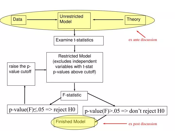
Unrestricted Model. Data. Theory. Examine t-statistics. ex ante discussion. Restricted Model (excludes independent variables with t-stat p-values above cutoff). raise the p-value cutoff. F-statistic. p-value(F)≤.05 => reject H0. p-value(F)>.05 => don’t reject H0. Finished Model.

E N D
Unrestricted Model Data Theory Examine t-statistics ex ante discussion Restricted Model (excludes independent variables with t-stat p-values above cutoff) raise the p-value cutoff F-statistic p-value(F)≤.05 => reject H0 p-value(F)>.05 => don’t reject H0 Finished Model ex post discussion
Standard Cross-Cultural Sample • World divided up into “culture regions,” one well-documented society picked from each of these, for total of 186 societies. • Over 2,000 variables gradually added. • Full range of human societies, so that any statement that claims to hold universally for humans can be tested.
Pct Monogamy for SCCS societies (local Getis) Smaller lighter circles have higher percent married women in polygynous marriages; larger darker circles have higher percent married women in monogamous marriages. Spatially smoothed.
% married women in monogamous marriages vs. political complexity In a box and whisker plot, the median is indicated by a heavy line, the box encloses the second and third quartile, and the whiskers extend out to the furthest datum within a distance of 1.5 times the box. The points beyond the whiskers are considered outliers.
% married women in monogamous marriages, by major language phylum and by religion
Pct. women in monogamous marriage vs. Pathogen Stress Y-axis: pct married women in monogamous marriages; x-axis: pathogen stress. Dotted red line is lowess smoother—high pathogen environments have less monogamy.
Two methodological issues • Galton’s problem (week 10) • Missing data (week 4)
First problem: Galton’s problem Observations not independent. • Common descent (language phylogeny) • Cultural borrowing (geographic distance, religion phylogeny) In regression context, Galton’s problem will cause biased coefficients and biased standard errors.
Galton’s problem example: Hypothesis: Drinking alcohol dampens the libido of religious specialists. alcohol wives Ecuador 1 0 Iran 0 2 Ireland 1 0 Morocco 0 3 Spain 1 0 Yemen 0 4 Pearson correlation= -0.9332565, p-value=0.0065 Adapted from Victor de Munck and Andrey Korotayev. 2000. “Cultural Units in Cross-Cultural Research.“ Ethnology 39(4): 335-348 An observed correlation between a pair of cultural traits across cultures could be due to the borrowing of the traits, as a package, from a common source (“horizontal transmission”), or could be due to their transmission, as a package, from a common ancestor (“vertical transmission”), or could be due to a true functional relationship.
Correcting for Galton’s problem (continued) Problem: The spatial weight matrices WR, WL and WD will be correlated with each other (societies with similar languages are usually physically proximate and have similar religions, as well), so that there is an identification problem with more than one spatial lag term. Solution: Create a new spatial matrix Woptimal= d*WD + r*WR + l*WL , where d+r+l=1. Make all possible matrices Woptimal using values (0,0.05,0.10,0.15,… , 0.85,0.90,0.95,1) for each of the weights (d,r,l). Estimate the model using each of the (211) weight matrices, recording the model R2. Retain the spatial weight matrix Woptimal which explains the highest variation of the dependent variable.
Second problem: Missing Data Societymarkinmarkoutmoneycommlandsharefood Nama Hottentot NA NA 1 NA NA Kung Bushmen 1 4 1 3 6 Thonga 4 4 3 3 6 Lozi 3 3 1 3 NA Mbundu NA NA 4 NA NA Suku 2 2 4 2 2 Two solutions: Listwise deletion Multiple imputation
Listwise deletion Societymarkinmarkoutmoneycommlandsharefood Nama Hottentot NA NA 1 NA NA Kung Bushmen 1 4 1 3 6 Thonga 4 4 3 3 6 Lozi 3313 NA Mbundu NA NA 4 NA NA Suku 2 2 4 2 2 • Lose three observations. Lose all of the information in the cells marked in red. • Of 186 societies, 156 would have been dropped using listwise deletion. No longer testing against the full range of human societies. Losing the big advantage of the SCCS. Probable sample selection bias.
Multiple imputation Replace missing values with imputed values, drawn from conditional distribution. Create several (5 to 10) new data sets with imputed values. Societymarkinmarkoutmoneycommlandsharefood Nama Hottentot 34 1 23 Kung Bushmen 1 4 1 3 6 Thonga 4 4 3 3 6 Lozi 3 3 1 3 6 Mbundu 45 4 31 Suku 2 2 4 2 2 Societymarkinmarkoutmoneycommlandsharefood Nama Hottentot 23 1 12 Kung Bushmen 1 4 1 3 6 Thonga 4 4 3 3 6 Lozi 3 3 1 3 4 Mbundu 35 4 53 Suku 2 2 4 2 2 Societymarkinmarkoutmoneycommlandsharefood Nama Hottentot 35 1 23 Kung Bushmen 1 4 1 3 6 Thonga 4 4 3 3 6 Lozi 3 3 1 3 5 Mbundu 26 4 42 Suku 2 2 4 2 2
Multiple imputation (continued) • Estimate model on each of the m imputed data sets • Combine m estimates using Rubin’s formulas, to get final estimate