Download
1 / 12
120 likes | 153 Views
Learn how to conduct Pareto analysis, interpret Pareto chart, and apply contingency analysis for quality improvement using practical steps and examples.

E N D
Sigma Quality Management -6 -4 -2 0 2 4 6 Pareto Analysis
Vilfredo Frederico Pareto & Joseph Juran Our Heroes!
Pareto Principle • A large fraction of power plant failures are due to boiler tube problems, • Seventy percent of assembly defects on irrigation sprinklers are due to problems inserting two components, • Over 75% of a printing company’s sales are to just three customers. • Wasted days in a hospital are due mainly to problems transferring patients to Skilled Nursing Facilities, • Delays receiving spare parts are most often associated with one vendor, • Over 90% of Mutual Fund transaction errors fall into four categories, • Sixty-five percent of employee injuries are back strains and sprains,
Pareto Analysis Process • What’s the Effect or Problem? • How Should the Effect be Measured? • How Can the Effect be Stratified? • What • When • Where • Who • What Does the Data Tell You? • “Zero-Type” Problems
Pareto Chart - Typographical Errors Total Count = 135 Percent Frequency 100 126 98% 90 87% 93% 112 79% 80 98 70 64% 84 60 70 50 56 40 48 - 36% 42 38 30 28 20 20 12 14 10 8 6 3 0 0 Missed Word Wrong Font Wrong Word Punctuation Misspelling Missed Sentence Duplicate Word The Pareto Chart
n COLUMNS A A ... A Total 1 2 n B X X ... X X 1 11 12 1n 1. m R OWS B X X ... X X 2 21 22 2n 2. B X X ... X X 3 31 32 3n 3. . . . ... . . B X X ... X X m m1 m2 mn m. Total X X ... X X .1 .2 .n .. Notation
Contingency Analysis - Steps 1. Establish the Hypothesis: • Null Hypothesis (Ho) - There is no relationship (i.e. independence exists) between Attributes A and B. • Alternative Hypothesis (Ha) - There is a relationship (i.e. dependence exists) between Attributes A and B. 2. Choose the Significance Level of the Test (). 3. Plan the Test: a) The Test Statistic is:
Contingency Analysis - Steps 3. Plan the Test: b) Determine the Rejection Region: Appendix A provides a table of the 2 distribution. Find the table value for(m - 1)(n - 1) degrees of freedom at the level of significance. For example, for a 4 row, 3 column contingency table, m = 4, n = 3 and the 2 value for 6 {(4 - 1) x (3 - 1) = 3 x 2 = 6} degrees of freedom at the 0.05 level of significance would be obtained from the look up table (this value is 12.59). The flu example is a 2 x 2 table, which therefore has {(2 - 1) x (2 - 1)} = 1 degree of freedom. From the table, then, the critical value (at the 0.05 level of significance) is 3.84.
Contingency Analysis - Steps 4. Collect the Data and calculate the Test Statistic. Data should then be collected and sorted into the cells and the expected counts table prepared. Now the test statistic can be calculated: 5. Draw the Conclusion. The last step is to compare the calculated value of the test statistic to the table value obtained from the chi-squared table. If the calculated value is greater than the table value, then it falls into the rejection region. The null hypothesis would then be rejected in favor of the alternative hypothesis.
Degrees a a a a = 0.2 = 0.1 = 0.05 = 0.01 of Freedom 1 1.64 2.71 3.84 6.64 2 3.22 4.61 5.99 9.21 3 4.6 4 6.25 7.82 11.34 4 5.99 7.78 9.49 13.28 5 7.29 9.24 11.07 15.09 6 8.56 10.65 12.59 16.81 7 9.80 12.02 14.07 18.48 8 11.03 13.36 15.51 20.90 9 12.24 14.68 16.92 21.67 10 13.44 15.98 18.31 23.21 11 14.63 17.28 19.68 24.73 12 15.81 18.55 21.03 26.22 13 16.99 19.81 22.36 27.69 14 18.15 21.06 23.69 29.14 15 19.31 22.31 25.00 30.58 16 20.47 23.54 26.30 32.00 17 21.62 24.77 27.59 33.41 18 22.76 25.99 28.89 34.81 19 23.90 27.20 30.14 36.19 20 25.04 28.41 31.41 37.57 25 30.68 34.38 37.65 44.31 30 36.25 40.26 43.77 50.89 Chi-Squared Table