Download
1 / 12
130 likes | 333 Views
Bivariate Linear Regression. Scatter plots of real world data rarely fit perfectly onto a straight line (or any other deterministic functional form.) e.g. Study time and exam grades.

E N D
Bivariate Linear Regression • Scatter plots of real world data rarely fit perfectly onto a straight line (or any other deterministic functional form.) e.g. Study time and exam grades. • y=a+bx is a deterministic relationship: knowing the value of x meaning knowing the value of y (assume we know the intercept and the slope). The correlation coefficient is 1 (or -1) in this case. e.g. Distance traveled = speed x time; fixing speed, there's a deterministic relationship between distance and time. • y=a+bx + e describes an imperfect linear relationship between two variables: the value of y is not completely determined by x, but is also affected by the “random error”, e. • In regression modeling, we try to fit a line through our scatter plot data, so that the (sum of squared) errors are minimized. • The straight line so obtained can then be used for interpretation of the relationship and for predictions.
Bivariate Linear Regression • Regression Model: E(yi) = a + bxi xi is the independent variable value for observation i. yi is the dependent/response variable value for observation i a and b are the intercept and slope of the straight line E(ei)=0 by model assumption • Meaning of b: a one unit increase in xi is associated with b units increase in E(yi). (If b is 0 in the population, then there is no relationship between xi and yi.). Meaning of a: E(yi) for xi=0. • The correlation coefficient, r, and the coefficient of x in the regression, b, are not the same thing, but their signs will agree. • How to find the “best” a and b? According to the “OLS” principle
Ordinary Least Squares (OLS) • Used to determine the “best” line that is as close as possible to the data points in the vertical (y) direction (since that is what we are trying to predict) • Least Squares: find the line that minimizes the sum of the squares of the vertical distances of the data points from the line (software does this for us. Soon...) • Property of OLS estimators: BLUE (best linear unbiased estimator)
Prediction Using Regression Line: Example (Husband and Wife's Ages) Hand, et.al., A Handbook of Small Data Sets, London: Chapman and Hall • The estimated regression model is E(y) = 3.6 + 0.97x E(y) is the average age of all husbands who have wives of age x • For all women aged 30, we predict the average husband age to be 32.7 years: 3.6 + (0.97)(30) = 32.7 years • If an individual wife’s age is 30. What would we predict her husband’s age to be? (Best prediction is still 32.7, since E(e)=0. But more uncertainty)
Hypothesis Testing: Is There a Relationship? • The estimated b value is based on one particular sample set, and so is the slope for the sample data. What is the slope in the population? • Testing population slope being zero in the population data (i.e., testing the hypothesis that there is no relationship between x and y): • Recall logic of hypothesis test • Under the null hypothesis, the sampling distribution of the estimated b/sd(b) is shown to follow the “Student-t” distribution (very similar to the normal, just thicker tails. A particular member of the family is characterized by one parameter, the degree of freedom) with n-2 degrees of freedom • Software routinely reports the p-value from the test
Goodness of Fit: the Coefficient of Determination (R2) • Measures how well the regression line fits the data • R2 equals r2 , the square of the correlation, and measures how much variation in the values of the response variable (y) is explained by the regression line • The distance between an observed Y and the mean of Y in the data set can be decomposed into two parts: from Y to E(Y) on the regression line, and from E(Y) to the mean of all Y. R2 is define as RSS/TSS. r=1: R2=1: regression line explains all (100%) of the variation in y r=.7: R2=.49: regression line explains almost half (50%) of the variation in y
Using Software • Stata: “regress” • Example: sysuse lifeexp; reg lexp safewater • egen ybar=mean(lexp) • twoway (scatter lexp safewater) (lfit lexp safewater) (line ybar safewater) • “Correlation and Regression Demo” applet at the book's website (explore the effect of outliers, for example.)
Using Linear Regression Model: Extrapolation Can Be Dangerous (e.g. What would be the presidential approval rate if the inflation rate rises to 200%?)
Caution: Correlation Does Not Imply Causation • Even very strong correlations may not correspond to a real causal relationship. • Correlation can be due to: • Explanatory variable a cause of response variable. e.g. x=meditation, y=health • “Response” variable a cause of “explanatory” variable. e.g. x=divorce, y=alcohol abuse • Both variables may result from a common cause (or there may be confounding). e.g. both divorce and alcohol abuse may result from an unhappy marriage. • The correlation may be merely a coincidence
Establishing Causality • A properly conducted experiment can establish the (lack of) causal connection • Other considerations lending support to arguments for a causal link: • A reasonable explanation for a cause and effect exists • The connection happens in repeated trials, and under varying conditions • Potential confounding factors are ruled out • Alleged cause precedes the effect in time