Download
1 / 8
80 likes | 177 Views
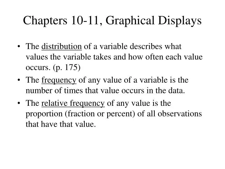
Chapters 10-11, Graphical Displays. The distribution of a variable describes what values the variable takes and how often each value occurs. (p. 175) The frequency of any value of a variable is the number of times that value occurs in the data.

E N D
Chapters 10-11, Graphical Displays • The distribution of a variable describes what values the variable takes and how often each value occurs. (p. 175) • The frequency of any value of a variable is the number of times that value occurs in the data. • The relative frequency of any value is the proportion (fraction or percent) of all observations that have that value.
Types of Variables • Categorical variable: Places an individual into one of several categories. (p. 178) • Examples: Gender, race, political party, zip code • Quantitative variable: Takes numerical values for which arithmetic operations make sense. (p. 178) • Examples: SAT score, number of siblings, cost of textbooks
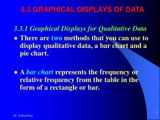
Graphs for categorical variables • Pie charts require relative frequencies since they display percentages and not raw data. The relative frequency of each category corresponds to the percent of the pie that is occupied by that category. • Bar graphs display data where the categories are on the horizontal axis and the frequencies (or relative frequencies) are on the vertical axis.
Graphs for quantitative variables Histograms: • The data are divided into classes of equal width and the number (or percentage) of observations in each class is counted. • Data scale is on the horizontal axis. • Frequency (or relative frequency) scale is on the vertical axis. • Bars are draw where base of each bar covers the class, height of each bar covers the frequency (or relative frequency).
Stemplots or Stem and Leaf Displays: • Separate each observation in a stem unit (all but the final rightmost digit of (rounded) data) and a leaf unit (the final digit of (rounded) data). • Write the stems in a vertical column, smallest to largest from top to bottom. • Write each leaf in the row to the right of its stem, in increasing order.
Histograms vs. Stemplots • Both are used to describe the distribution of data. • Stemplots display actual data values. • Stemplots are used for small data sets (less than 100 values). • Histogram can be constructed for larger data sets.
Common Distributional Shapes: • A symmetric distribution is one where both sides about the center line are approximately mirror images of each other. • A skewed distribution is one where one side of the center line contains more data than the other. (p. 202) • Skewed to the right: The right side of the histogram extends much farther than the left side. • Skewed to the left: The left side of the histogram extends much farther than the right side.
Common Distributional Shapes: • A bimodal distribution has two humps where much of the data lies. • All classes occur with approximately the same frequency in a uniform distribution. • An outlier in any graph of data is an individual observation that falls outside the overall pattern of the graph. (p. 201)