Download
1 / 41
410 likes | 545 Views
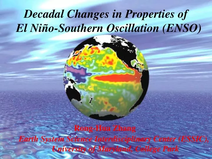
Decadal Changes in Properties of El Niño-Southern Oscillation (ENSO) Rong-Hua Zhang Earth System Science Interdisciplinary Center (ESSIC), University of Maryland, College Park. Observations => El Nino Property shift in the late 1970s.

E N D
Decadal Changes in Properties of El Niño-Southern Oscillation (ENSO) Rong-Hua Zhang Earth System Science Interdisciplinary Center (ESSIC), University of Maryland, College Park
Observations => El Nino Property shift in the late 1970s Pre-shift period: 2-3 yr oscillation; westward propagation of SSTA; weak SSTA in far east. Equ. Pacific Post-shift period: 4-5 yr oscillation; eastward propagation of SSTA; strong SSTA in far east. Equ. Pacific What caused the decadal changes ?
Mechanisms for Decadal ENSO Changes • Random factors Stochastic forcing, Nonlinearity, Residual effect, … • Deterministic factors Changes in mean climate states: Atmosphere: wind stress Ocean : the thermocline depth, stratification, SST, … Changes in thespatial structure of subsurface ocean thermal fields
The role of atmos stochastic forcing (SF) A null hypothesis for causing ENSO irregularity Significant effects on ENSO & its changes ENSO characteristics, Predictability, … Limitations to previous studies: Random factor systematic & coherent way in Obs? Focusing on amplitude & period; propagation ? Decadal subsurface temperature changes? ICM : Zebiak-Cane model: Te specified HCM: Statistical + OGCM What are the respective roles relative to Te ?
Observed decadal changes in ocean temperature in the Pacificin the late 1970sData: World Ocean Database at NODC/NOAA (Levitus et al.)Decadal variability in the Pacific basin: 1. The Midlatitude/extratropics 2. The tropics 3. Oceanic connections from the midlatitude/extratropics to the tropics
157W-22N 172W-2N 157W-2N
Decadal change in entrainment temperature (Te) & its role in ENSO Hypothesis: Subsurface thermal structure change => ENSO changes Testing using coupled models The Temperature of subsurface water entrained into the mixed layer (Te) Decadal changes in the structure of Te
Te: The Temperature of subsurface water entrained into the mixed layer Wind stress (τ) SST mixed layer Te Te We
SST anomaly model Te: The Temperature of subsurface water entrained into the mixed layer
Outline • Introduction • Intermediate ocean model (IOM) with an empirical parameterization for Te • The Role of Subsurface Entrainment Temperature (Te) (1) Intermediate coupled model ( ICM; Zhang and Busalacchi, 2005) Ocean: Intermediate ocean model (IOM) + an SST anomaly model + Te Atmospheric wind stress (τ) model: SVD-based statistical (2) Hybrid coupled model (HCMAGCM ) Ocean: The IOM as in the ICM Atmosphere: AGCM (ECHAM4.5) • The respective roles of atmospheric stochastic forcing (SF) & Te • Summary
Intermediate ocean model (IOM): Ocean dynamical model + a SST anomaly model Linear part: Non-linear part Vertical modal decomposition
SST anomaly model Te: The Temperature of subsurface water entrained into the mixed layer
Te Parameterization scheme 1. Cane-Zebiak scheme 2. Empirical parameterization scheme
SST anomaly model Te: The Temperature of subsurface water entrained into the mixed layer
An empirical model for the Temperature of water Entrained (Te) into the mixed layer Historical data: simulated & observed Forced ocean model run => currents, pressure fields ( Sea level (SL) ) • Inverse modeling of Te Obs. SST fields etc. => SST anomaly model => Te • Statistical relationships based on history: SLTe SVD-based analysis of covariance between SL and Te Given SL from ocean model => Te => SST calculation Nothing could be better than this procedure in simulating SSTA !!
Data Sets and Construction of Te models • SST (Reynolds et al.): 1950-1999 • Dynamical ocean model run forced by NCEP: 1960-1999 => mean fields; anomaly fields: sea level (SL) etc Inverse modeling of SSTA equation => Te ________________________________________________________________________ • Te model construction: SL Te Seasonally invariant ( 1 model for all months); 1963-1996 1963-1979 1980-1996
Intermediate coupled model (ICM): IOM + statistical anomaly model Atmos: A SVD-based wind stress model: Observed SSTAs Wind stress anomalies (τ) from ECHAM4.5 24 member ensemble mean Ocean:IOM with Te
Hybrid coupled model (HCM):IOM + an AGCM Atmosphere: The European Center + The Max Planck Institute for Meteorology (MPI) Atmospheric GCM (ECHAM4.5) T42; 19 layers Ocean:IOM with Te
ICMHCMAGCM(Intermediate coupled model) (Hybrid coupled model)
Realizations of atmos stochastic forcing (SF) in the coupled models Wind stress response: Signal + Noise (SF) SST HCM: AGCM + IOM with Te SF: implicitly included ICM: statistical + IOM with Te (1) Signal part in wind stress anomalies (No SF) (2) Both parts: SF explicitly taken into account
Construction of τsignal&τSF Wind stress ( τ ) : Signal+ noise (stochastic forcing) obs. SSTAs - AGCM (ECHAM4.5) 24 ensemble meanHCM (ECHAM4.5 + IOM) Residual A first order autocorrelation model (AR1) τSignal + τSF =>Used in ICM
The ICM experiments τSignal τSignal + τSF Te model:63-96; 63-79; 80-96 τ model : 63-96; 63-79; 80-96 Te63-79, Te80-96
The HCMAGCM experiments Te63-79 , Te80-96
Coupled modeling experiments on the effects of Te & SFon ENSO properties
Oceanic processes involved Off-equatorialTe SST Hori adv. Vert adv. mixed layer Te thermolcine
Summary • Demonstrate anew factor determining the El Nino properties • Different modulating effects of SF & Te: SF Irregularity of ENSO amplitude & oscillation periods Te Phase propagation
Implication for observations ExplainEl Nino Property shift in the late 1970s Pre-shift period: 2-3 yr oscillation; westward propagation of SSTA; weak SSTA in far east. Equ. Pacific Post-shift period: 4-5 yr oscillation; eastward propagation of SSTA; strong SSTA in far east. Equ. Pacific
Implications for coupled modeling Common biases with OGCM-based Coupled Models: Quas-biennial (~2 yr) oscillation; westward propagation of SSTA on equ.; weak SSTA in far eastern equatorial Pacific Improvements: better Te simulations


![El Niño Southern Oscillation [ENSO]](https://cdn1.slideserve.com/1597810/el-ni-o-southern-oscillation-enso-dt.jpg)