Download
1 / 47
520 likes | 959 Views
Chapter 5: Process Scheduling. Chapter 5: Process Scheduling. Basic Concepts Scheduling Criteria Scheduling Algorithms (6) Multiple-Processor Scheduling Thread Scheduling OS Examples Algorithm Evaluation. Basic Concepts.

E N D
Chapter 5: Process Scheduling • Basic Concepts • Scheduling Criteria • Scheduling Algorithms (6) • Multiple-Processor Scheduling • Thread Scheduling • OS Examples • Algorithm Evaluation
Basic Concepts • In a multiprogramming system, multiple processes exist concurrently in main memory. • Each process alternates between using a processor and waiting for some event to occur, such as the completion of an I/O operation. • The processor is kept busy by executing one process while the others wait. • The key to multiprogramming is scheduling. • Process Scheduling is • the basis of multi-programmed operating system • a fundamental function of operating-system.
Basic Concepts • In a single-processor system • Only one process can run at a time • Any others must waituntil the CPU is free and can be rescheduled. • When the running process goes to the waiting state, • the OS may select another process to assign CPU to improve CPU utilization. • Every time one process has to wait, another process can take over use of the CPU • Process scheduling is • to select a process from the ready queue and assign the CPU
Diagram of Process State from ch.3 • It is important to realize that only one process can be running on any processor at any instant. • Many processes may be ready and waiting states.
Process Scheduling from ch.3 • The process selection is carried out by the short-term scheduler (or CPU scheduler). • The scheduler selects a process from the processes in memory that are ready to execute and allocates the CPU to that process.
CPU - I/O burst Cycle • Process execution consists of • a cycle of CPU execution (CPU burst) and I/O wait (I/O burst) • Process alternate between these two states • Process execution begins with a CPU burst, which is followed by an I/O burst, and so on. • Eventually, the final CPU burst ends with an system call to terminate execution. • CPU burst distribution of a process • varies greatly from process to process and from computer to computer
CPU burst time I/O burst time CPU burst time CPU burst time Alternating Sequence of CPU & I/O Bursts
Histogram of CPU-burst Times • CPU burst distribution is generally characterized • as exponential or hyper-exponential • with large number of short CPU burst and small number of long CPU burst • I/O bound process has many short CPU bursts • CPU bound process might have a few long CPU bursts.
Process Scheduler • selects one of the processes in memory that are ready to execute, and allocates the CPU to the selected process. • CPU scheduling decisions may take place when a process: 1. switches from running to waiting state: I/O request, invocation of wait() for the termination of other process 2.switches from running to ready state: when interrupt occurs 3.switches from waiting to ready: at completion of I/O 4.terminates
Process Scheduler(cont.) • Scheduling under 1 and 4 is non-preemptive • Scheduling under 2 and 3 is preemptive
Non-preemptive vs. Preemptive • Non-preemptive scheduling • Once the CPU has been allocated to a process, the process keeps the CPU until it releases the CPU • either byterminating or by switching to the waiting state. • used by Windows 3.x • Preemptive scheduling • Current running process can be switched with another at any time • because interrupt can occur at any time • Most of modern OS provides this scheme. (Windows XP, Max OS, UNIX)
Dispatcher • Dispatcher module gives control of the CPU to the process selected by the short-term scheduler; this involves: • switching context • switching to user mode • jumping to the proper location in the user program to restart that program • Dispatch latency–time it takes for the dispatcher to stop one process and start another running CPU-scheduling function ? ?
Scheduling Criteria • Based on the scheduling criteria, the performance of various scheduling algorithm could be evaluated. • Different scheduling algorithms have different properties. • CPU utilization–keep the CPU as busy as possible. i.e., ratio (%) of the amount of time while the CPU was busy per time unit. • Throughput– # of processes that complete their execution per time unit. • Turnaround time– the interval from the time of submission of a process to the time of completion. Sum of the periods spent waiting to get into memory, waiting in the ready queue, executing on the CPU, and doing I/O • Waiting time– Amount of time a process has been waiting in the ready queue, which is affected by scheduling algorithm • Response time– In an interactive system, amount of time it takes from when a request was submitted until the first response is produced, not output (for time-sharing environment)
Optimization Criteria • It is desirable to maximize: • The CPU utilization • The throughput • It is desirable to minimize: • The turnaround time • The waiting time • The response time • However in some circumstances, it is desirable to optimize the minimum or maximum values rather than the average. • Interactive systems, it is more important to minimize the variance in the response time than minimize the average response time.
Process Scheduling Algorithms • First-Come, First-Served Scheduling (FCFS) • Shortest-Job-First Scheduling (SJF) • Priority Scheduling • Round-Robin Scheduling • Our measure of comparison is the average waiting time.
P1 P2 P3 0 24 27 30 First-Come, First-Served (FCFS) Scheduling • The process that request the CPU first is allocated the CPU first. ProcessBurst Time(ms) P1 24 P2 3 P3 3 • Suppose that the processes arrive in the order: P1 , P2 , P3 The Gantt Chart for the schedule is: • Waiting time for P1 = 0; P2 = 24; P3 = 27 • Average waiting time: (0 + 24 + 27)/3 = 17ms
P2 P3 P1 0 3 6 30 FCFS Scheduling Suppose that the processes arrive in the order P2 , P3 , P1 • The Gantt chart for the schedule is: • Waiting time for P1 = 6;P2 = 0; P3 = 3 • Average waiting time: (6 + 0 + 3)/3 = 3 • Much better than previous case
FCFS Scheduling • FCFS scheduling algorithm is non-preemptive • Once the CPU has been allocated to a process, that process keeps the CPU until it releases the CPU, either by terminating or by requesting I/O. • is particularly troublesome for time-sharing systems (response time ). • Convoy effect (short process behind long process)occurs: • When one CPU-bound process with long CPU burst and many I/O-bound process which short CPU burst. • All I/O bound process waits for the CPU-bound process to get off the CPU while I/O is idle • All I/O- and CPU- bound processes executes I/O operation while CPU is idle. • results in low CPU and device utilization
Shortest-Job-First (SJF) Scheduling • SJF associates with each process the length of its next CPU burst. • use these lengths to schedule the process with the shortest time • Two schemes: • non-preemptive– once CPU given to the process it cannot be preempted until completes its CPU burst • preemptive– if a new process arrives with CPU burst length less than remaining time of current executing process, preempt. This scheme is knownas the Shortest-Remaining-Time-First (SRTF) • SJF is optimal– gives minimum average waiting time for a given set of processes
P3 P2 P4 P1 3 9 16 24 0 Example of Non-Preemptive SJF ProcessBurst Time P1 6 P2 8 P3 7 P4 0 3 • SJF scheduling chart (non-preemptive) • Average waiting time = (3 + 16 + 9 + 0) / 4 = 7
P1 P2 P3 P2 P4 P1 11 16 0 2 4 5 7 Example of Preemptive SJF (SRTF) ProcessArrival TimeBurst Time P1 0.0 7 P2 2.0 4 P3 4.0 1 P4 5.0 4 • SJF (preemptive) • Average waiting time = (9 + 1 + 0 +2)/4 = 3
How do we know the length of the next CPU burst? • by computing an approximation of the length of the next CPU burst (estimate the length of the next CPU burst) • can be done by using the length of previous CPU bursts, using exponential averaging • The value of tn contains our most recent information. • n+1 stores the past history • The parameter controls the relative weight of recent and past history in our prediction.
Prediction of the Length of the Next CPU Burst • In this example, 0 = 10, = ½ , t1=6 • 1 = x t0 + (1- ) x 0 = ½ x 6 + ½x 10 = 8 • 2 = x t2 + (1- ) x 1 = ½ x 4 + ½x 8 = 6
Examples of Exponential Averaging • = 0 • n+1 = n = n-1 = n-2 . … = 0 • Recent history does not count • = 1 • n+1 = tn • Only the actual last CPU burst counts i.e., the most recent CPU burst • If we expand the formula, we get: n+1 = tn+ (1 - ) tn - 1+ … + (1 - )j tn-j+ … + (1 - )n +1 0 • Since both and (1 - ) are less than or equal to 1, each successive term has less weight than its predecessor
Priority Scheduling • A priority number (integer) is associated with each process • The CPU is allocated to the process with the highest priority (smallest integer highest priority) • Preemptive • Non-preemptive
Example 1 of Non-Preemptive Priority ProcessBurst TimePriority arrival time P1 10 3 0 P2 1 1 0 P3 2 4 0 P4 1 5 0 P5 5 2 0 • Priority Scheduling (non-preemptive) • Average waiting time = (0 + 1 + 6 + 16 + 18)/5 = 8.2 P2 P5 P4 P1 P3 16 6 18 19 0 1
P1 P2 P5 P4 P3 10 3 14 17 19 0 Example 2 of Non-Preemptive Priority scheduling chart (non-preemptive) Total Waiting time = (0-0) + (3-1) +(17-4) + (14-2) + (10-6) = 0+2+13+12+4=31 ms Average waiting time= 31/5 = 6.2 ms Total Turnaround time= (3-0) + (10-1) + (19-4) + (17-2) + (14- 6) = 50 ms Average Turnaround time= 50/5 = 10ms
P1 P2 P5 P4 P2 P3 P1 0 1 6 10 13 15 17 19 Example of Preemptive Priority scheduling chart (preemptive) Process P1 preempted by p2 because p2 has higher priority Total Waiting time = (0-0+17-1) + (1-1+13-6) +(15-4) + (10-2) + (6-6) =42ms Average waiting time= 42/5= 8.4 ms Total Turnaround time= (19-0) + (15-1) + (17-4) + (13-2) + (10-6) = 61ms Average Turnaround time= 61/5 = 12.2ms
Priority Scheduling • SJF is a priority scheduling where priority is the predicted next CPU burst time • Problem Starvation– low priority processes may never execute • Solution Aging– as time progresses, increase the priority of the process 0 127
Round Robin (RR) Scheduling • It is similar to FCFS scheduling, but preemption is added to enable the system to switch between process. • Each process gets a small unit of CPU time (time quantum), usually 10-100 milliseconds. • After this time has elapsed, the process is preempted and added to the end of the ready queue.
If CPU cycle (CPU burst time ) > time quantum • Job is preempted and put at the end of the READY Q • If CPU cycle < time quantum • If job finished • resources released • If interrupted by I/O request • Info saved in PCB • Linked at end of appropriate I/O queue • When I/O complete, job returns to READY Q
Example of RR with Time Quantum = 4 ProcessBurst Time Arrival Time P1 24 0 P2 3 0 P3 3 0 The Gantt chart is: P1 P2 P3 P1 P1 P1 P1 P1 0 10 14 18 22 26 30 4 7 Total Waiting time = (0-0+10-4) + (4-0) +(7-0) =17ms Context switch ??? Average waiting time= 17/3= 5.66 ms Total Turnaround time= (30-0) + (7-0) + (10-0) = 47ms Average Turnaround time= 47/5= 9.4 ms
P1 P2 P3 P4 P5 P2 P3 P4 P5 0 7 17 27 37 47 50 60 64 74 P3 P5 P5 79 89 99 Example of RR with Time Quantum = 10 • The Gantt chart is: Total Waiting time = (0-0) + (7-1 + 47-17 )+(17-5+ 50-27+ 74- 60)+(27-6+60-37)+ (37-8+64-47+79-64 ) = 180 ms Average waiting time= 180/5= 36 ms Total Turnaround time= (7-0) + (50-1) + (79-5)+(64-6)+(99-8) = 279ms Average Turnaround time= 279/5= 55.8 ms
Round Robin (RR) Scheduling • Performance depends on the size of the time quantum. • If the time quantum is extremely large, the RR policy is the same as the same as the FCFS policy • If the time quantum is extremely small (say 1 millisec) , the RR approach is called processor sharing i.e., provides high concurrency: each of n processes has its own processor running at 1/n the speed of the real processor
Time Quantum and Context Switch Time a b c • In (a) the job finishes before the time quantum expires. • In (b) and (c), the time quantum expires first, interrupting the job • The effect of context switching on the performance of RR scheduling, for example one process of 10 time quantum. • quantum = 12 time units, finished in less than 1 time quantum • quantum = 6 time units, requires 2 quanta, 1 context switch • quantum = 1 time units, requires 10 quanta, 9 context switch
Round Robin (RR) Scheduling • Thetime quantum qmust be large with respect to context switch, otherwise overhead is too high • If the context switching time is 10% of the time quantum, then about 10% of the CPU time will be spent in context switching • Most modern OS have time quanta ranging from 10 to 100milliseconds, • The time required for a context switch is typically less than 10 microseconds; thus the context-switch time is a small fraction of the time quantum.
Turnaround Time varies with the Time Quantum • Theturnaround timedepends on the size ofthe time quantum • The average turnaroundtime of a set of processes • dose not necessarily improve • as the time quantum size • Increased. • The average turnaroundtime can be improvedif most processes finish their next CPU burst in a single time quantum.
Scheduling Algorithm with multi-Queues • Multi-level Queue Scheduling • Multi-level FeedbackQueue Scheduling
Multilevel Queue • Ready queue is partitioned into separate queues:foreground (interactive)background (batch) • The processes are permanently assigned to one queue, generally based on some property, or process type. • Each queue has its own scheduling algorithm • foreground–RR • background–FCFS • Scheduling must be done between the queues • Fixed priority scheduling - serve all from foreground then from background, Possibility of starvation. • Time slicescheduling– each queue gets a certain amount of CPU time which it can schedule amongst its processes; i.e., 80% to foreground in RR, 20% to background in FCFS
Multilevel Queue Scheduling • No process in the batch queue could run unless the queues with high priority were all empty. • If an interactive editing process entered the ready queue while a batch process was running, the batch process would be preempted.
Multilevel Feedback Queue • A process can move between the various queues; aging can be implemented in this way • Multilevel-feedback-queue scheduler defined by the following parameters: • number of queues • scheduling algorithms for each queue • method used to determine when to upgrade a process • method used to determine when to demote a process • method used to determine which queue a process will enter when that process needs service
Example of Multilevel Feedback Queue • Three queues: • Q0–RR with time quantum 8 milliseconds • Q1–RR time quantum 16 milliseconds • Q2–FCFS • Scheduling • A new job enters queue Q0which is servedRR. When it gains CPU, job receives 8 milliseconds. If it does not finish in 8 milliseconds, job is moved to queue Q1. • At Q1 job is again served RR and receives 16 additional milliseconds. If it still does not complete, it is preempted and moved to queue Q2. • The job is serverd based on FCFS in queue Q2
Summary • CPU scheduling is the task of selecting a waiting process from the ready queue and allocating the CPU to it. • The CPU is allocated to the selected process by the dispatcher. • FCFS scheduling is simple, cause short processes to wait for long time • SJF scheduling is provably optimal, providing the shortest averaging waiting time. But predicting the length of the next CPU bursts is difficult. • Priority scheduling allocates the CPU to the heights priority process. • Both priority and SJF may suffer from starvation. Aging is a technique to prevent starvation. • RR scheduling is more appropriate for a time-shared system. • Major problem of RR scheduling is the selection of the time quantum. • FCFS is non-preemptive, RR is preemptive, SJF and Priority may be preemptive and non-preemptive. • Multilevel queue allows different scheduling algorithm for each queue. • Multilevel feedback queue allow process to move from one queue to another.