Download
1 / 40
400 likes | 569 Views
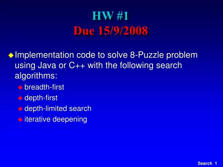
HW #1 Due 15/9/2008. Implementation code to solve 8-Puzzle problem using Java or C++ with the following search algorithms: breadth-first depth-first depth-limited search iterative deepening. Blind Search.

E N D
HW #1Due 15/9/2008 • Implementation code to solve 8-Puzzle problem using Java or C++ with the following search algorithms: • breadth-first • depth-first • depth-limited search • iterative deepening
Blind Search • Depth-first search and breadth-first search are examples of blind (or uninformed) search strategies. • Breadth-first search produces an optimal solution (eventually, and if one exists), but it still searches blindly through the state-space. • Neither uses any knowledge about the specific domain in question to search through the state-space in a more directed manner. • If the search space is big, blind search can simply take too long to be practical, or can significantly limit how deep we're able to look into the space. • A search strategy is defined by picking the order of node expansion
Informed Search - Overview • Heuristic Search • Best-First Search Approach • Greedy • A* • Heuristic Functions • Local Search and Optimization • Hill-climbing • Simulated Annealing • Local Beam • Genetic Algorithms
Informed Search • relies on additional knowledge about the problem or domain • frequently expressed through heuristics. • used to distinguish more promising paths towards a goal • may be mislead, depending on the quality of the heuristic • in general, performs much better than uninformed search • but frequently still exponential in time and space for realistic problems
Informed Search (Cont.) • find a solution more quickly, • find solutions even when there is limited time available, • often find a better solution, since more profitable parts of the state-space can be examined, while ignoring the unprofitable parts. • A search strategy which is better than another at identifying the most promising branches of a search-space is said to be more informed.
Best-First Search • relies on an evaluation function f(n) that gives an indication of how useful it would be to expand a node • family of search methods with various evaluation functions • usually gives an estimate of the distance to the goal • often referred to as heuristics in this context • the node with the lowest value is expanded first • Fringe is ordered by f(n) • the name is a little misleading: the node with the lowest value for the evaluation function is not necessarily one that is on an optimal path to a goal function BEST-FIRST-SEARCH(problem, EVAL-FN) returnssolution fringe := queue with nodes ordered by EVAL-FN return TREE-SEARCH(problem, fringe)
Greedy Best-First Search • minimizes the estimated cost to a goal • expand the node that seems to be closest to a goal • utilizes a heuristic function as evaluation function • f(n) = h(n) = estimated cost from the current node to a goal • heuristic functions are problem-specific • e.g., fSLD(n) = straight-line distance • often straight-line distance for route-finding and similar problems • often better than depth-first. function GREEDY-SEARCH(problem) returnssolution return BEST-FIRST-SEARCH(problem, h)
Greedy Best-First Search Snapshot Initial 9 1 Visited Fringe Current 7 7 2 3 Visible Goal 6 5 5 6 4 5 6 7 Heuristics 7 7 5 4 3 2 4 5 6 8 9 10 11 12 13 14 15 8 7 6 5 4 3 2 1 0 1 2 3 4 5 6 7 16 17 18 19 20 21 22 23 24 25 26 27 28 29 30 31 Fringe: [13(4), 7(6), 8(7)] + [24(0), 25(1)]
Route Finding 374 253 366 329
Greedy best-first search example So is Arad->Sibiu-> Fagaras->Bucharest optimal?
Greedy search, evaluation • Completeness: NO • Check on repeated states • Minimizing h(n) can result in false starts, e.g. Iasi to Fagaras.
Greedy search, evaluation • An obvious problem with greedy search is that it doesn't take account of the cost so far, so it isn't optimal, and can wander into dead-ends, like depth-first search. 0 Cost Max local minimum = looping Initial State Goal
A* Search • combines greedy and uniform-cost search to find the (estimated) cheapest path through the current node • f(n) = g(n) + h(n) = path cost + estimated cost to the goal from n • heuristics must be admissible • h(n) never overestimate the cost to reach the goal • very good search method, but with complexity problems function A*-SEARCH(problem) returnssolution return BEST-FIRST-SEARCH(problem, g+h)
A* Search Evaluation Function: F(n) = g(n) + h(n) Estimated cost of cheapest path from node n to goal Path cost from root to node n
A* Snapshot 9 Initial 9 1 Visited Fringe 4 3 11 10 Current 7 7 2 3 Visible 7 2 2 4 Goal 10 13 6 5 5 6 4 5 6 7 Edge Cost 9 2 5 4 4 4 3 6 9 Heuristics 7 11 12 7 5 4 3 2 4 5 6 f-cost 10 8 9 10 11 12 13 14 15 3 4 7 2 4 8 6 5 4 3 4 2 8 3 9 2 13 13 8 7 6 5 4 3 2 1 0 1 2 3 4 5 6 7 16 17 18 19 20 21 22 23 24 25 26 27 28 29 30 31 Fringe: [2(4+7), 7(3+4+6), 13(3+2+3+4)] + [24(3+2+4+4+0), 25(3+2+4+3+1)]
A* Snapshot with all f-Costs Initial 9 1 Visited Fringe 4 3 11 10 Current 7 7 2 3 Visible 7 2 2 4 Goal 17 11 10 13 6 5 5 6 4 5 6 7 Edge Cost 9 2 5 4 4 4 3 6 9 Heuristics 7 20 21 14 13 11 12 18 22 7 5 4 3 2 4 5 6 f-cost 10 8 9 10 11 12 13 14 15 3 4 7 2 4 8 6 5 4 3 4 2 8 3 9 2 24 24 29 23 18 19 18 16 13 13 14 13 25 21 31 25 3 8 7 6 5 4 3 2 1 0 1 2 4 5 6 7 16 17 18 19 20 21 22 23 24 25 26 27 28 29 30 31
A* Properties • the value of f never decreases along any path starting from the initial node • this property can be used to draw contours • regions where the f-cost is below a certain threshold • the better the heuristics h, the narrower the contour around the optimal path
A* Snapshot with Contour f=11 Initial 9 1 Visited Fringe 4 3 11 10 Current 7 7 2 3 Visible 7 2 2 4 Goal 17 11 10 13 6 5 5 6 4 5 6 7 Edge Cost 9 2 5 4 4 4 3 6 9 Heuristics 7 20 21 14 13 11 12 18 22 7 5 4 3 2 4 5 6 f-cost 10 8 9 10 11 12 13 14 15 3 4 7 2 4 8 6 5 4 3 4 2 8 3 9 2 Contour 24 24 29 23 18 19 18 16 13 13 14 13 25 21 31 25 3 8 7 6 5 4 3 2 1 0 1 2 4 5 6 7 16 17 18 19 20 21 22 23 24 25 26 27 28 29 30 31
A* Snapshot with Contour f=13 Initial 9 1 Visited Fringe 4 3 11 10 Current 7 7 2 3 Visible 7 2 2 4 Goal 17 11 10 13 6 5 5 6 4 5 6 7 Edge Cost 9 2 5 4 4 4 3 6 9 Heuristics 7 20 21 14 13 11 12 18 22 7 5 4 3 2 4 5 6 f-cost 10 8 9 10 11 12 13 14 15 3 4 7 2 4 8 6 5 4 3 4 2 8 3 9 2 Contour 24 24 29 23 18 19 18 16 13 13 13 25 21 31 25 3 8 7 6 5 4 3 2 1 0 1 4 5 6 7 16 17 18 19 20 21 22 23 24 25 27 28 29 30 31 14 2 26
A* Search • A* expands nodes in increasing f value • Gradually adds f-contours of nodes
Optimality of A* • A* will find the optimal solution • the first solution found is the optimal one • A* is optimally efficient • no other algorithm is guaranteed to expand fewer nodes than A* • A* is not always “the best” algorithm • optimality refers to the expansion of nodes • other criteria might be more relevant • it generates and keeps all nodes in memory • improved in variations of A*
Complexity of A* • the number of nodes within the goal contour search space is still exponential • with respect to the length of the solution • better than other algorithms, but still problematic • frequently, space complexity is more severe than time complexity • A* keeps all generated nodes in memory
Memory-Bounded Search • search algorithms that try to conserve memory • most are modifications of A* • iterative deepening A* (IDA*) • Recursive best-first search (RBFS) • simplified memory-bounded A* (SMA*)
Iterative Deepening A* (IDA*) • explores paths within a given contour (f-cost limit) in a depth-first manner • this saves memory space because depth-first keeps only the current path in memory • but it results in repeated computation of earlier contours since it doesn’t remember its history • was the “best” search algorithm for many practical problems for some time • does have problems with difficult domains
Recursive Best-First Search • similar to best-first search, but with lower space requirements • O(bd) instead of O(bm) • it keeps track of the best alternative to the current path • best f-value of the paths explored so far from predecessors of the current node • if it needs to re-explore parts of the search space, it knows the best candidate path • still may lead to multiple re-explorations
RBFS: best alternative over fringe nodes, which are not children: do I want to back up? RBFS changes its mind very often in practice. This is because the f=g+h become more accurate (less optimistic) as we approach the goal. Hence, higher level nodes have smaller f-values and will be explored first.
Simplified Memory-Bounded A* (SMA*) • uses all available memory for the search • drops nodes from the queue when it runs out of space • those with the highest f-costs • If there is a tie (equal f-values) we first delete the oldest nodes first. • complete if there is enough memory for the shortest solution path • often better than A* and IDA* • but some problems are still too tough • trade-off between time and space requirements
Heuristics for Searching • for many tasks, a good heuristic is the key to finding a solution • prune the search space • move towards the goal
Example: 8-Puzzle Average solution cost for a random puzzle is 22 moves Branching factor is about 3 Empty tile in the middle -> four moves Empty tile on the edge -> three moves Empty tile in corner -> two moves 322 is approx 3.1e10 Get rid of repeated states 181440 distinct states Heuristic Functions 8-Puzzle
Heuristic Functions 8-Puzzle • h1=the number of misplaced tiles • h2=the sum of the Manhattan distances of the tiles from their goal positions • h1 = 7 • h2 = 4+0+3+3+1+0+2+1 = 14
Heuristic Functions 8-Puzzle • h1=0 • h2=0 • h1=2 • h2=8 • h1=2 • h2=2