Download
1 / 66
720 likes | 1.22k Views
Statistical Process Control. Operations Management Dr. Ron Tibben-Lembke. Designed Size. 10 11 12 13 14 15 16 17 18 19 20. Natural Variation. 14.5 14.6 14.7 14.8 14.9 15.0 15.1 15.2 15.3 15.4 15.5.

E N D
Statistical Process Control Operations Management Dr. Ron Tibben-Lembke
Designed Size 10 11 12 13 14 15 16 17 18 19 20
Natural Variation 14.5 14.6 14.7 14.8 14.9 15.0 15.1 15.2 15.3 15.4 15.5
Theoretical Basis of Control Charts Properties of normal distribution 95.5% of allX fall within ± 2
Theoretical Basis of Control Charts Properties of normal distribution 99.7% of allX fall within ± 3
Skewness • Lack of symmetry • Pearson’s coefficient of skewness: Positive Skew > 0 Negative Skew < 0 Skewness = 0
Kurtosis • Amount of peakedness or flatness Kurtosis = 0 Kurtosis > 0 Kurtosis < 0
Design Tolerances • Design tolerance: • Determined by users’ needs • UTL -- Upper Tolerance Limit • LTL -- Lower Tolerance Limit • Eg: specified size +/- 0.005 inches • No connection between tolerance and • completely unrelated to natural variation.
LTL UTL 6 Process Capability and 6 LTL UTL 3 • A “capable” process has UTL and LTL 3 or more standard deviations away from the mean, or 3σ. • 99.7% (or more) of product is acceptable to customers
LTL LTL UTL UTL LTL UTL Process Capability Capable Not Capable LTL UTL
Process Capability • Specs: 1.5 +/- 0.01 • Mean: 1.505 Std. Dev. = 0.002 • Are we in trouble?
Process Capability • Specs: 1.5 +/- 0.01 • LTL = 1.5 – 0.01 = 1.49 • UTL = 1.5 + 0.01 = 1.51 • Mean: 1.505 Std. Dev. = 0.002 • LCL = 1.505 - 3*0.002 = 1.499 • UCL = 1.505 + 0.006 = 1.511 Process Specs 1.49 1.51 1.511 1.499
Capability Index • Capability Index (Cpk) will tell the position of the control limits relative to the design specifications. • Cpk>= 1.0, process is capable • Cpk< 1.0, process is not capable
Process Capability, Cpk • Tells how well parts produced fit into specs Process Specs 3 3 LTL UTL
Process Capability • Tells how well parts produced fit into specs • For our example: • Cpk= min[ 0.015/.006, 0.005/0.006] • Cpk= min[2.5,0.833] = 0.833 < 1 Process not capable
Process Capability: Re-centered • If process were properly centered • Specs: 1.5 +/- 0.01 • LTL = 1.5 – 0.01 = 1.49 • UTL = 1.5 + 0.01 = 1.51 • Mean: 1.5 Std. Dev. = 0.002 • LCL = 1.5 - 3*0.002 = 1.494 • UCL = 1.5 + 0.006 = 1.506 Process Specs 1.49 1.494 1.506 1.51
If re-centered, it would be Capable Process Specs 1.49 1.494 1.506 1.51
Packaged Goods • What are the Tolerance Levels? • What we have to do to measure capability? • What are the sources of variability?
Production Process Make Candy Make Candy Make Candy Mix Package Put in big bags Make Candy Mix % Wrong wt. Wrong wt. Make Candy Make Candy Candy irregularity
Processes Involved • Candy Manufacturing: • Are M&Ms uniform size & weight? • Should be easier with plain than peanut • Percentage of broken items (probably from printing) • Mixing: • Is proper color mix in each bag? • Individual packages: • Are same # put in each package? • Is same weight put in each package? • Large bags: • Are same number of packages put in each bag? • Is same weight put in each bag?
Your Job • Write down package # • Weigh package and candies, all together, in grams and ounces • Write down weights on form • Optional: • Open package, count total # candies • Count # of each color • Write down • Eat candies • Turn in form and empty complete wrappers for weighing
Peanut Color Mix website • Brown 17.7% 20% • Yellow 8.2% 20% • Red 9.5% 20% • Blue 15.4% 20% • Orange 26.4% 10% • Green 22.7% 10%
Plain Color Mix Class website • Brown 12.1% 30% • Yellow 14.7% 20% • Red 11.4% 20% • Blue 19.5% 10% • Orange 21.2% 10% • Green 21.2% 10%
So who cares? • Dept. of Commerce • National Institutes of Standards & Technology • NIST Handbook 133 • Fair Packaging and Labeling Act
Package Weight • “Not Labeled for Individual Retail Sale” • If individual is 18g • MAV is 10% = 1.8g • Nothing can be below 18g – 1.8g = 16.2g
Goal of Control Charts • collect and present data visually • allow us to see when trend appears • see when “out of control” point occurs
X Process Control Charts • Graph of sample data plotted over time UCL Process Average ± 3 LCL Time
X Process Control Charts • Graph of sample data plotted over time UCL Assignable Cause Variation LCL Natural Variation Time
Definitions of Out of Control • No points outside control limits • Same number above & below center line • Points seem to fall randomly above and below center line • Most are near the center line, only a few are close to control limits • 8 Consecutive pts on one side of centerline • 2 of 3 points in outer third • 4 of 5 in outer two-thirds region
Attributes vs. Variables Attributes: • Good / bad, works / doesn’t • count % bad (P chart) • count # defects / item (C chart) Variables: • measure length, weight, temperature (x-bar chart) • measure variability in length (R chart)
Attribute Control Charts • Tell us whether points in tolerance or not • p chart: percentage with given characteristic (usually whether defective or not) • np chart: number of units with characteristic • c chart: count # of occurrences in a fixed area of opportunity (defects per car) • u chart: # of events in a changeable area of opportunity (sq. yards of paper drawn from a machine)
p Chart Control Limits # Defective Items in Sample i Sample iSize
p Chart Control Limits z = 2 for 95.5% limits; z = 3 for 99.7% limits # Defective Items in Sample i Sample iSize # Samples
p Chart Control Limits z = 2 for 95.5% limits; z = 3 for 99.7% limits # Defective Items in Sample i Sample iSize # Samples
p Chart Example You’re manager of a 500-room hotel. You want to achieve the highest level of service. For 7 days, you collect data on the readiness of 200 rooms. Is the process in control (use z = 3)? © 1995 Corel Corp.
p Chart Hotel Data No. No. NotDayRoomsReadyProportion 1 200 16 16/200 = .080 2 200 7 .035 3 200 21 .105 4 200 17 .085 5 200 25 .125 6 200 19 .095 7 200 16 .080
p Chart Control Limits 16 + 7 +...+ 16
p Chart Solution 16 + 7 +...+ 16
p Chart Solution 16 + 7 +...+ 16
p Chart UCL LCL
R Chart • Type of variables control chart • Interval or ratio scaled numerical data • Shows sample ranges over time • Difference between smallest & largest values in inspection sample • Monitors variability in process • Example: Weigh samples of coffee & compute ranges of samples; Plot
Hotel Example You’re manager of a 500-room hotel. You want to analyze the time it takes to deliver luggage to the room. For 7 days, you collect data on 5 deliveries per day. Is the process in control?
Hotel Data DayDelivery Time 1 7.30 4.20 6.10 3.45 5.55 2 4.60 8.70 7.60 4.43 7.62 3 5.98 2.92 6.20 4.20 5.10 4 7.20 5.10 5.19 6.80 4.21 5 4.00 4.50 5.50 1.89 4.46 6 10.10 8.10 6.50 5.06 6.94 7 6.77 5.08 5.90 6.90 9.30
7.30 + 4.20 + 6.10 + 3.45 + 5.55 5 Sample Mean = R &X Chart Hotel Data Sample DayDelivery TimeMean Range 1 7.30 4.20 6.10 3.45 5.55 5.32
Sample Range = 7.30 - 3.45 R &X Chart Hotel Data Sample DayDelivery TimeMean Range 1 7.30 4.20 6.10 3.45 5.55 5.32 3.85 Largest Smallest
R &X Chart Hotel Data Sample DayDelivery TimeMean Range 1 7.30 4.20 6.10 3.45 5.55 5.32 3.85 2 4.60 8.70 7.60 4.43 7.62 6.59 4.27 3 5.98 2.92 6.20 4.20 5.10 4.88 3.28 4 7.20 5.10 5.19 6.80 4.21 5.70 2.99 5 4.00 4.50 5.50 1.89 4.46 4.07 3.61 6 10.10 8.10 6.50 5.06 6.94 7.34 5.04 7 6.77 5.08 5.90 6.90 9.30 6.79 4.22