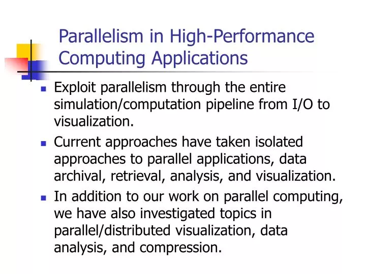
Parallelism in High-Performance Computing Applications

1. Parallelism in High-Performance Computing Applications • Exploit parallelism through the entire simulation/computation pipeline from I/O to visualization. • Current approaches have taken isolated approaches to parallel applications, data archival, retrieval, analysis, and visualization. • In addition to our work on parallel computing, we have also investigated topics in parallel/distributed visualization, data analysis, and compression.

2. Scalable Parallel Volume Visualization • Highly optimized shear-warp algorithm forms the basis for parallelization. • Optimizations include image and object space coherence, early termination, compression. • Parallel (MPI-based) formulation on SP is shown to scale to 128 processors and achieve frame rates in excess of 15 fps for UNC Brain dataset (256x256x167).

3. Parallel Shear-Warp • Data Partitioning: • Sheared volume partitioning • Compositing: • Software compositing/binary aggregation • Load Balancing: • Coherence in object movement -- use previous frame to load balance current frame.

4. Data/Computation Partitioning

5. Performance Notes • Only scan-lines corresponding to incremental shear need to be communicated between frames. • Since relative shear is not large, this communication overhead is small.

6. Performance Notes • MPI version tested on up to 128 processors of an IBM SP (112MHz PowerPC 604), among other platforms. • Datasets scaling from 128 x 128 x 84 to 256 x 256 x 167 (UNC Brain/Head datasets).

7. Performance Notes. All rendering times are in milliseconds and include compositing time.

8. Data Analysis Techniques for Very High Dimensional Data • Datasets from simulations/physical processes can have extremely high dimensionality and large volume. • This data is also typically sparse. • Interpreting this data requires scalable techniques for detection of dominant and deviant patterns. • Handling large discrete-valued datasets • Extracting co-occurrences between events • Summarizing data in an error-bounded fashion • Finding concise representations for summary data

9. Background • Singular Value Decomposition (SVD) [Berry et.al., 1995] • Decompose matrix into A=USVT • U and V orthogonal matrices, Sdiagonal with singular values • Used for Latent Semantic Indexing in Information Retrieval • Truncate decomposition to compress data

10. Background • Semi-Discrete Decomposition (SDD) [Kolda and O’Leary, 1998] • Restrict entries of U and V to {-1,0,1} • Requires very small amount of storage • Can perform as well as SVD in LSI using less than one-tenth the storage • Effective in finding outlier clusters • works well for datasets containing a large number of small clusters

11. Rank-1 Approximations x : presence vector y : pattern vector

12. Problem:Given discrete matrix Amxn , find discrete vectors xmx1 and ynx1 to Minimize = number of non-zeros in the error matrix solve for x to Maximize Heuristic: Fix y, set Discrete Rank-1 Approximation Iteratively solve for x and y until no improvement possible

13. - At any step, given rank-one approximation AxyT, split A into A1and A0 based on rows: - if x(i)=0 row i goes to A0 - Stop when - Hamming radius of A1, maximum of the Hamming distances of A1pattern vector, is less then some threshold - All rows of A are present in A1 (if A1does not satisfy Hamming radius condition, can split A1 based on Hamming distances) Recursive Algorithm - if x(i)=1 row i goes to A1

14. Effectiveness of Analysis

15. Effectiveness of Analysis

16. runtime vs # columns runtime vs # rows runtime vs # nonzeros Run-time Scalability • Rank-1 approximation requires O(nz(A)) time • Total run-time at each level in the recursive tree cannot exceed • this since total # of nonzeros at each level is at most nz(A) • Run-time is linear in nz(A)