Finite Element Method for 1D Acoustic Wave Equation

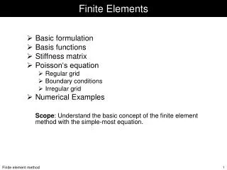
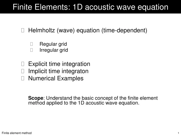
1. Finite Elements: 1D acoustic wave equation Helmholtz (wave) equation (time-dependent) Regular grid Irregular grid Explicit time integration Implicit time integraton Numerical Examples Scope: Understand the basic concept of the finite element method applied to the 1D acoustic wave equation.

2. Acoustic wave equation in 1D How do we solve a time-dependent problem such as the acoustic wave equation? where v is the wave speed. using the same ideas as before we multiply this equation with an arbitrary function and integrate over the whole domain, e.g. [0,1], and after partial integration .. we now introduce an approximation for u using our previous basis functions...

3. Weak form of wave equation note that now our coefficients are time-dependent! ... and ... together we obtain which we can write as ...

4. Time extrapolation M b A mass matrix stiffness matrix ... in Matrix form ... ... remember the coefficients c correspond to the actual values of u at the grid points for the right choice of basis functions ... How can we solve this time-dependent problem?

5. Time extrapolation ... let us use a finite-difference approximation for the time derivative ... ... leading to the solution at time tk+1: we already know how to calculate the matrix A but how can we calculate matrix M?

6. Mass matrix ... let’s recall the definition of our basis functions ... i=1 2 3 4 5 6 7 + + + + + + + h1 h2 h3 h4 h5 h6 ... let us calculate some element of M ...

7. Mass matrix – some elements Diagonal elements: Mii, i=2,n-1 ji i=1 2 3 4 5 6 7 + + + + + + + h1 h2 h3 h4 h5 h6 xi hi-1 hi

8. Matrix assembly Mij Aij % assemble matrix Aij A=zeros(nx); for i=2:nx-1, for j=2:nx-1, if i==j, A(i,j)=1/h(i-1)+1/h(i); elseif i==j+1 A(i,j)=-1/h(i-1); elseif i+1==j A(i,j)=-1/h(i); else A(i,j)=0; end end end % assemble matrix Mij M=zeros(nx); for i=2:nx-1, for j=2:nx-1, if i==j, M(i,j)=h(i-1)/3+h(i)/3; elseif j==i+1 M(i,j)=h(i)/6; elseif j==i-1 M(i,j)=h(i)/6; else M(i,j)=0; end end end

9. Numerical example

10. Implicit time integration ... let us use an implicit finite-difference approximation for the time derivative ... ... leading to the solution at time tk+1: How do the numerical solutions compare?

11. Summary The time-dependent problem (wave equation) leads to the introduction of the mass matrix. The numerical solution requires the inversion of a system matrix (it may be sparse). Both explicit or implicit formulations of the time-dependent part are possible.