Download
1 / 62
920 likes | 1.48k Views
Financial Options. Topics in Chapter. What is a financial option? Options Terminology Profit and Loss Diagrams Where and How Options Trade? The Binomial Model Black-Scholes Option Pricing Model. 1. What is a financial option?.

E N D
Topics in Chapter • What is a financial option? • Options Terminology • Profit and Loss Diagrams • Where and How Options Trade? • The Binomial Model • Black-Scholes Option Pricing Model
1. What is a financial option? • An option is a contract which gives its holder the right, but not the obligation, to buy (or sell) an asset at some predetermined price within a specified period of time. • It does not obligate its owner to take any action. It merely gives the owner the right to buy or sell an asset.
2.Option Terminology • A call option gives you the right to buy within a specified time period at a specified price • The owner of the option pays a cash premium to the option seller in exchange for the right to buy
2. Option Terminology • A put option gives you the right to sell within a specified time period at a specified price • It is not necessary to own the asset before acquiring the right to sell it
2. Option Terminology • Strike (or exercise) price: The price stated in the option contract at which the security can be bought or sold. • Expiration date: The last date the option can be exercised.
2. Option Terminology • Exercise value: The value of a call option if it were exercised today = • Max[0, Current stock price - Strike price] • Note: The exercise value is zero if the stock price is less than the strike price. • Option price: The market price of the option contract.
2. Option Terminology • The price of an option has two components: • Intrinsic value: • For a call option equals the stock price minus the striking price • For a put option equals the striking price minus the stock price • Time value equals the option premium minus the intrinsic value
3. Profit and Loss Diagrams • For the Disney JUN 22.50 Call buyer: Maximum profit is unlimited Breakeven Point = $22.75 $0 -$0.25 Maximum loss $22.50
3. Profit and Loss Diagrams • For the Disney JUN 22.50 Call writer: Maximum profit Breakeven Point = $22.75 $0.25 $0 Maximum loss is unlimited $22.50
3. Profit and Loss Diagrams • For the Disney JUN 22.50 Put buyer: Maximum profit = $21.45 Breakeven Point = $21.45 $0 -$1.05 Maximum loss $22.50
Call Time Value Diagram Option value 30 25 20 15 10 5 Market price Exercise value 5 10 15 20 25 30 35 40 Stock Price
4. Where and How Options Trade? • Options trade on four principal exchanges: • Chicago Board Options Exchange (CBOE) • American Stock Exchange (AMEX) • Philadelphia Stock Exchange • Pacific Stock Exchange
4. Where and How Options Trade? • AMEX and Philadelphia Stock Exchange options trade via the specialist system • All orders to buy or sell a particular security pass through a single individual (the specialist) • The specialist: • Keeps an order book with standing orders from investors and maintains the market in a fair and orderly fashion • Executes trades close to the current market price if no buyer or seller is available
4. Where and How Options Trade? • CBOE and Pacific Stock Exchange options trade via the marketmaker system • Competing marketmakers trade in a specific location on the exchange floor near the order book official • Marketmakers compete against one another for the public’s business
4. Where and How Options Trade? • Any given option has two prices at any given time: • The bid price is the highest price anyone is willing to pay for a particular option • The asked price is the lowest price at which anyone is willing to sell a particular option
5. The Binomial Model • The value of the replicating portfolio at time T, with stock price ST, is ΔST + (1+r)T*B where Δ is the # of share s and B is cash invested • At the prices ST = Sou and ST = Sod, a replicating portfolio will satisfy (Δ * Sou ) + (B * (1+r)T )= Cu (Δ * Sod ) + (B * (1+r)T )= Cd Solving for Δ and B Δ = (Cu - Cd) / (So(u –d) ) B = (Cu - (Δ * Sou) )/ (1+r)T and substitute in C = ΔSo + B to get the option price
5. The Binomial Model • Stock assumptions: • Current price: So = $27 • In next 6 months, stock can either • Go up by factor of u = 1.41 • Go down by factor of 0.71 • Call option assumptions • Expires in t = 6 months = 0.5 years • Exercise price: X = $25 • Risk-free rate: 6% a year a day (r = 0.06/365 a day)
Ending "up" price = fu = Sou = $38.07 Option payoff: Cu = MAX[0, fu−X] = $13.07 Currentstock priceSo = $27 Ending “down" price = = fd = Sod = $19.17 Option payoff: Cd = MAX[0, fd −X] = $0.00 u = 1.41d = 0.71X = $25 5. The Binomial Model
Ending "up" price = fu = $38.07 Ending "up" stock value = Δ*fu = $26.33Option payoff: Cu = MAX[0,fu −X] = $13.07Portfolio's net payoff = Δ*fu - Cu = $13.26 Currentstock priceSo = $27 Ending “down" stock price = fd = $19.17 Ending “down" stock value = Δ*fd = $13.26Option payoff: Cd = MAX[0,fd −X] = $0.00Portfolio's net payoff = Δ*fd - Cd = $13.26 u = 1.41d = 0.71X = $25Δ = 0.6915 5. Riskless Portfolio’s Payoffs at Call’s Expiration: $13.26
5. Create portfolio by writing 1 option and buying Δ shares of stock. • Portfolio payoffs: • Stock is up: Δ * Sou − Cu • Stock is down: Δ * Sod − Cd
5. The Hedge Portfolio with a Riskless Payoff • Set payoffs for up and down equal, solve for number of shares: • Δ = (Cu− Cd) / (So(u− d)) • B = (Cu − (Δ * Sou) )/ (1+r)T = - (Portfolio's net payoff )/ (1+r)T • In our example: • Δ = ($13.07 − $0) / $27(1.41− 0.71) =0.6915 • B = - $13.26/(1 + 0.06 / 365 )365*0.5 = -$12.87
5. The Hedge Portfolio with a Riskless Payoff • Option Price C =ΔSo + B =0.6915($27) + (-$12.87) = $18.67 − $12.87 = $5.80 If the call option’s price is not the same as the cost of the replicating portfolio, then there will be an opportunity for arbitrage. Option Premium C + (Commission)
5. Arbitrage Example • Suppose the option sells for $6. • You can write option, receiving $6. • Create replicating portfolio for $5.80, netting $6.00 −$5.80 = $0.20. • Arbitrage: • You invested none of your own money. • You have no risk (the replicating portfolio’s payoffs exactly equal the payoffs you will owe because you wrote the option. • You have cash ($0.20) in your pocket.
5. Arbitrage and Equilibrium Prices • If you could make a sure arbitrage profit, you would want to repeat it (and so would other investors). • With so many trying to write (sell) options, the extra “supply” would drive the option’s price down until it reached $5.80 and there were no more arbitrage profits available. • The opposite would occur if the option sold for less than $5.80.
5. Multi-Period Binomial Pricing • If you divided time into smaller periods and allowed the stock price to go up or down each period, you would have a more reasonable outcome of possible stock prices when the option expires. • This type of problem can be solved with a binomial lattice. • As time periods get smaller, the binomial option price converges to the Black-Scholes price, which we discuss in later slides.
6. Black-Scholes • Fischer Black and Myron Scholes published the derivation and equation of the Black-Scholes Option Pricing Model in 1973 under several assumptions. • Bottom line: options of traded stocks are fundamentally priced
6. Black-Scholes Option Pricing Model • The stock underlying the call option provides no dividends during the call option’s life. • There are no transactions costs for the sale/purchase of either the stock or the option. • Risk-free rate, rRF, is known and constant during the option’s life. (More...)
6. Black-Scholes Option Pricing Model • Security buyers may borrow any fraction of the purchase price at the short-term risk-free rate. • No penalty for short selling and sellers receive immediately full cash proceeds at today’s price. • Call option can be exercised only on its expiration date. • Security trading takes place in continuous time, and stock prices move randomly in continuous time.
6. Black Scholes Equation • Integration of statistical and mathematical models • For example in the standard Black-Scholes model, the stock price evolves as • dS = μ(t)Sdt + σ(t)SdWt. • where μ is the drift parameter and σ is the implied volatility • To sample a path following this distribution from time 0 to T, we divide the time interval • into M units of length δt, and approximate the Brownian motion over the interval dt • by a single normal variable of mean 0 and variance δt. • The price f of any derivative (or option) of the stock S is a solution of the • following partial-differential equation:
6. Black-Scholes Option Pricing Model • The Black-Scholes OPM:
6. Black-Scholes Option Pricing Model • Variable definitions: • C = theoretical call premium • S = current stock price • t = time in years until option expiration • K = option striking price • R = risk-free interest rate
6. Black-Scholes Option Pricing Model • Variable definitions (cont’d): • = standard deviation of stock returns • N(x) = probability that a value less than “x” will occur in a standard normal distribution • ln = natural logarithm • e = base of natural logarithm (2.7183)
6. Black-Scholes Option Pricing Model Example Stock ABC currently trades for $30. A call option on ABC stock has a striking price of $25 and expires in three months. The current risk-free rate is 5%, and ABC stock has a standard deviation of 0.45. According to the Black-Scholes OPM, but should be the call option premium for this option?
6. Black-Scholes Option Pricing Model Example (cont’d) Solution: We must first determine d1 and d2:
6. Black-Scholes Option Pricing Model Example (cont’d) Solution (cont’d):
6. What is the value of the following call option according to the OPM? • Assume: • N = P = $27 • X = $25 • rRF = 6% • t = 0.5 years • σ = 0.49
6. First, find d1 and d2. d1 = {ln($27/$25) + [(0.06 + 0.492/2)](0.5)} ÷ {(0.49)(0.7071)} d1 = 0.4819 d2 = 0.4819 - (0.49)(0.7071) d2 = 0.1355
6. Second, find N(d1) and N(d2) • N(d1) = N(0.4819) = 0.6851 • N(d2) = N(0.1355) = 0.5539 • Note: Values obtained from Excel using NORMSDIST function. For example: • N(d1) = NORMSDIST(0.4819)
6. Third, find value of option. VC = $27(0.6851) - $25e-(0.06)(0.5)(0.5539) = $19.3536 - $25(0.97045)(0.6327) = $5.06
What impact do the following parameters have on a call option’s value? • Current stock price: Call option value increases as the current stock price increases. • Strike price: As the exercise price increases, a call option’s value decreases.
6. Impact on Call Value • Option period: As the expiration date is lengthened, a call option’s value increases (more chance of becoming in the money.) • Risk-free rate: Call option’s value tends to increase as rRF increases (reduces the PV of the exercise price). • Stock return variance: Option value increases with variance of the underlying stock (more chance of becoming in the money).
6. Negative Affects • Myron Scholes was a partner of Long-Term Capital Management (LTCM) established in 1994. • LTCM would use models and experienced investing knowledge to pick differences in short and long securities, profiting from the small margin. • In 1998 the firm had $5B in equity and $125B in liability • August 17, 1998 Russia devalues the rouble and suspended $13.5B of it’s Treasury Bonds, causing LTCM’s equity to decrease drastically, ever increasing it’s leverage ratio • In order to prevent a stock market crash due to the outflux of investors and banks from LTCM’s funds the Federal Reserve organized a $3.5 B rescue effort to take over LTCM’s management • Had LTCM lost leverage, all banks and creditors would pull out of other firms – including Salomon Brothers, Merrill Lynch.