Understanding High Dimensional Data and Principal Components Analysis

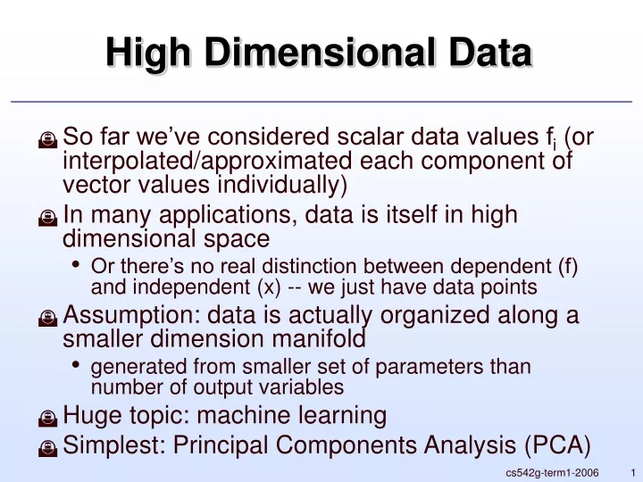
1. High Dimensional Data • So far we’ve considered scalar data values fi (or interpolated/approximated each component of vector values individually) • In many applications, data is itself in high dimensional space • Or there’s no real distinction between dependent (f) and independent (x) -- we just have data points • Assumption: data is actually organized along a smaller dimension manifold • generated from smaller set of parameters than number of output variables • Huge topic: machine learning • Simplest: Principal Components Analysis (PCA) cs542g-term1-2006

2. PCA • We have n data points from m dimensions: store as columns of an mxn matrix A • We’re looking for linear correlations between dimensions • Roughly speaking, fitting lines or planes or hyperplanes through the origin to the data • May want to subtract off the mean value along each dimension for this to make sense cs542g-term1-2006

3. Reduction to 1D • Assume data points fit through a line through the origin (1D subspace) • In this case, say line is along unit vector u. (m-dimensional vector) • Each data point should be a multiple of u (call the scalar multiples wi): • That is, A would be rank-1: A=uwT • Problem in general: find rank-1 matrix that best approximates A cs542g-term1-2006

4. The rank-1 problem • Use Least-Squares formulation again: • Clean it up: take w=v with ≥0 and |v|=1 • u and v are the first principal components of A cs542g-term1-2006

5. Solving the rank-1 problem • Remember trace version of Frobenius norm: • Minimize with respect to sigma first: • Then plug in to get a problem for u and v: cs542g-term1-2006

6. Finding u • First look at u: • AAT is symmetric, thus has a complete set of orthonormal eigenvectors X, eigenvectors mu • Write u in this basis: • Then maximizing: • Obviously pick u to be the eigenvector with largest eigenvalue cs542g-term1-2006

7. Finding v • Write the thing we’re maximizing as: • Same argument gives v the eigenvector corresponding to max eigenvalue of ATA • Note we also have cs542g-term1-2006

8. Generalizing • In general, if we expect problem to have subspace dimension k, we want the closest rank-k matrix to A • That is, express the data points as linear combinations of a set of k basis vectors(plus error) • We want the optimal set of basis vectors and the optimal linear combinations: cs542g-term1-2006

9. Finding W • Take the same approach as before: • Set gradient w.r.t. W equal to zero: cs542g-term1-2006

10. Finding U • Plugging in W=ATU we get • AAT is symmetric, hence has a complete set of orthogonormal eigenvectors, say columns of X, and eigenvalues along the diagonal of M (sorted in decreasing order): cs542g-term1-2006

11. Finding U cont’d • Our problem is now: • Note X and U are both orthogonal, so is XTU, which we can call Z: • Simplest solution: set Z=(I 0)T which means thatU is the first k columns of X(first k eigenvectors of AAT) cs542g-term1-2006

12. Back to W • We can write W=V∑T for an orthogonal V, and square kxk ∑ • Same argument as for U gives that V should be the first k eigenvectors of ATA • What is ∑? • From earlier rank-1 case we know • Since U*1 and V*1 are unit vectors that achieve the 2-norm of AT and A, we can derive that first row and column of ∑ is zero except for diagonal. cs542g-term1-2006

13. What is ∑ • Subtract rank-1 matrix U*1∑11V*1T from A • zeros matching eigenvalue of ATA or AAT • Then we can understand the next part of ∑ • End up with ∑ a diagonal matrix, containing the squareroots of the first k eigenvalues of AAT or ATA (they’re equal) cs542g-term1-2006

14. The Singular Value Decomposition • Going all the way to k=m (or n) we get the Singular Value Decomposition (SVD) of A • A=U∑VT • The diagonal entries of ∑ are called the singular values • The columns of U (eigenvectors of AAT) are the left singular vectors • The columns of V (eigenvectors of ATA) are the right singular vectors • Gives a formula for A as a sum of rank-1 matrices: cs542g-term1-2006

15. Cool things about the SVD • 2-norm: • Frobenius norm: • Rank(A)= # nonzero singular values • Can make a sensible numerical estimate • Null(A) spanned by columns of U for zero singular values • Range(A) spanned by columns of V for nonzero singular values • For invertible A: cs542g-term1-2006

16. Least Squares with SVD • Define pseudo-inverse for a general A: • Note if ATA is invertible, A+=(ATA)-1AT • I.e. solves the least squares problem] • If ATA is singular, pseudo-inverse defined:A+b is the x that minimizes ||b-Ax||2 and of all those that do so, has smallest ||x||2 cs542g-term1-2006

17. Solving Eigenproblems • Computing the SVD is another matter! • We can get U and V by solving the symmetric eigenproblem for AAT or ATA, but more specialized methods are more accurate • The unsymmetric eigenproblem is another related computation, with complications: • May involve complex numbers even if A is real • If A is not normal (AAT≠ATA), it doesn’t have a full basis of eigenvectors • Eigenvectors may not be orthogonal… Schur decomp • Generalized problem: Ax=Bx • LAPACK provides routines for all these • We’ll examine symmetric problem in more detail cs542g-term1-2006

18. The Symmetric Eigenproblem • Assume A is symmetric and real • Find orthogonal matrix V and diagonal matrix D s.t. AV=VD • Diagonal entries of D are the eigenvalues, corresponding columns of V are the eigenvectors • Also put: A=VDVT or VTAV=D • There are a few strategies • More if you only care about a few eigenpairs, not the complete set… • Also: finding eigenvalues of an nxn matrix is equivalent to solving a degree n polynomial • No “analytic” solution in general for n≥5 • Thus general algorithms are iterative cs542g-term1-2006