Understanding Discrete Fourier Transform for Signal Analysis

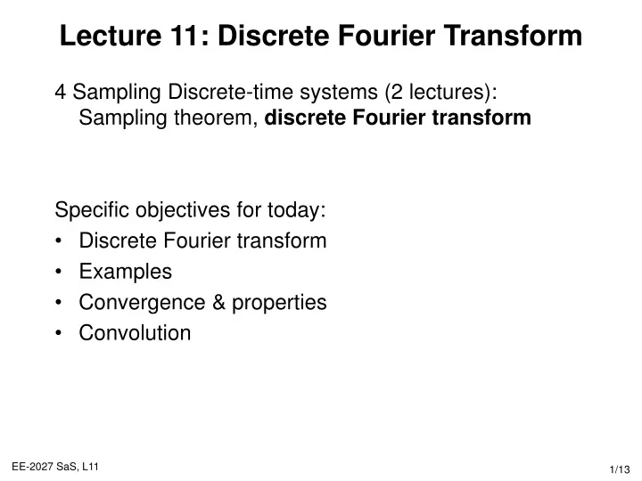
1. Lecture 11: Discrete Fourier Transform • 4Sampling Discrete-time systems (2 lectures): Sampling theorem, discrete Fourier transform • Specific objectives for today: • Discrete Fourier transform • Examples • Convergence & properties • Convolution

2. Lecture 11: Resources • Core reading • SaS, O&W, 5.1-5.4 • Background reading • MIT Lectures 9 and 10

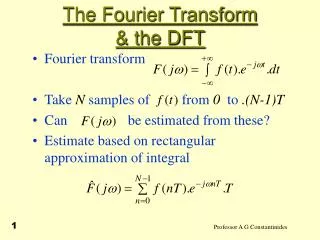
3. Reminder: CT Fourier Transform • CT Fourier transform maps a time domain frequency signal to the frequency domain via • The Fourier transform is used to • Analyse the frequency content of a signal • Design a system/filter with particular properties • Solve differential equations in the frequency domain using algebraic operators • Note that the transform/integral is not defined for some signals (infinite energy)

4. Derivation of the DT Fourier Transform • By analogy with the CT Fourier transform, we might “guess” • This is because tn, & the integral operator represents the limit of a sum as the sum’s width tends to zero. • X(ejw) is periodic of period 2p, so is ejwn. Try substituting into the inverse Fourier transform with integral over 2p: • which is the original DT signal.

5. Discrete Time Fourier Transform • The DT Fourier transform analysis and synthesis equations are therefore: • The function X(ejw) is referred to as the discrete-time Fourier transform and the pair of equations are referred to as the Fourier transform pair • X(ejw) is sometimes referred to as the spectrum of x[n] because it provides us with information on how x[n] is composed of complex exponentials at different frequencies • It converges when the signal is absolutely summable

6. Example 1: 1st Order System, Decay Power • Calculate the DT Fourier transform of the signal: • Therefore: stable system a=0.8

7. Example 2: Rectangular Pulse • Consider the rectangular pulse • and the Fourier transform is N1=2

8. Example 3: Impulse Signal • Fourier transform of the DT impulse signal is

9. Properties: Periodicity, Linearity & Time • The DT Fourier transform is always periodic with period 2p, because • X(ej(w+2p)) = X(ejw) • It is relatively straightforward to prove that the DT Fourier transform is linear, i.e. • Similarly, if a DT signal is shifted by n0 units of time

10. Convolution in the Frequency Domain • Like continuous time signals and systems, the time-domain convolution of two discrete time signals can be represented as the multiplication of the Fourier transforms • If x[n], h[n] and y[n] are the input, impulse response and output of a discrete-time LTI system so, by convolution, • y[n] = x[n]*h[n] • Then • Y(ejw) = X(ejw)H(ejw) • The proof is analogous to proof used for the convolution of continuous time Fourier transforms • Convolution in the discrete time domain is replaced by multiplication in the frequency domain.

11. Example: 1st Order System • Consider an LTI system with impulse response • h[n]=anu[n], |a|<1 • and the system input is • x[n]=bnu[n], |b|<1 • The DT Fourier transforms are: • So • Expressing as partial fractions, assuming ab: • and spotting the inverse Fourier transform

12. Lecture 11: Summary • Apart from a slightly difference, the Fourier transform of a discrete time signal is equivalent to the continuous time formulae • They have similar properties to the continuous time Fourier transform for linearity, time shifts, differencing and accumulation • The main result is that like continuous time signals and systems, convolution in the time domain is replaced by multiplication in the frequency domain. • Y(ejw) = X(ejw)H(ejw)

13. Lecture 11: Exercises • Theory • SaS, O&W, 5.1-5.3, 5.19