Computation on Arbitrary Surfaces

1. Computation on Arbitrary Surfaces Brandon Lloyd COMP 258 October 2002

2. Computation on Arbitrary Surfaces • Mathematical framework for Euclidean geometry enables us to perform important operations • Usually peformed on regular grid • Triangle meshes have irregular connectivity, hence irregular sampling • Triangle meshes are general 2-manifolds

3. Computation on Arbitrary Surfaces • Displaced Subdivision Surfaces • Multi-resolution signal processing on meshes • Texture synthesis on meshes

4. Displaced Subdivision Surfaces • Aaron Lee, Henry Moreton and Hughes Hoppe in SIGGRAPH 2000. • The idea is to use a scalar-valued displacement over a smooth domain mesh Control mesh Smooth domain surface Displaced subdivision surface

5. Representation • Control mesh for domain surface • Regular scalar displacement mesh • Subdivided along with the control mesh to produce a continuous displacement function • Uses parameterization of the domain surface • Displacement map may be used as a bump map

6. Conversion Process • Obtain the control mesh • Optimize the control mesh to more closely resemble original • Sample displacement map Original mesh Displaced subdivision surface

7. Simplifying the Control Mesh • Done with edge collapses • Map vertex normals from neighborhood of candidate edge collapse to Gauss sphere • Disallow collapse if original normals are not enclosed in spherical triangle

8. Optimizing the Domain Surface • Move vertices of control mesh to more accurately fit the original mesh • Densely sample original mesh and minimize least squared distances • Affects normals, but does not produce noticeable problems Initial control mesh Optimized control mesh

9. Sampling the Displacement Map • Perform subdivision on optimized control mesh • Intersect ray formed by point and normal with original mesh • Store distance in displacement map Subdivided Domain surface Displacement field

10. Applications • Compression – The displacement map contains small, similar values • Editing – simply modify the scalar field • Animation – easier to kinematics with control mesh

11. Compression Results

12. Prefilter and downsample image Ln to produce Ln-1 Burt-Adelson Pyramids 2

13. Prefilter and downsample image Ln to produce Ln-1 Upsample Ln-1and subtract from Ln Burt-Adelson Pyramids 2 2

14. Prefilter and downsample image Ln to produce Ln-1 Upsample Ln-1and subtract from Ln Repeat till you reach L0 Burt-Adelson Pyramids 2 2

15. Prefilter and downsample image Ln to produce Ln-1 Upsample Ln-1and subtract from Ln Repeat till you reach L0 The result is an image pyramid with a frequency subband at each level Burt-Adelson Pyramids 2 2

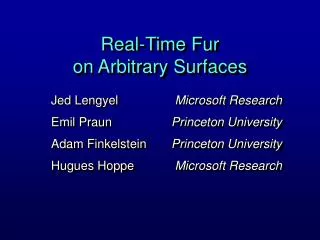
16. Multiresolution Signal Processing for Meshes • Igor Guskov, Wim Sweldens and Peter Schröder in SIGGRAPH 1999. • Generalizes basic signal processing tools such as downsampling, upsampling, and filters to irregular triangle meshes • Uses a non-uniform relaxation procedure for geometric smoothing • Smoothing combined with hierarchical algorithms are used to build subdivision and pyramid methods

17. Importance of Smoothness • Geometric smoothness measures variance in triangle normals. • Geometric smoothness implies that there exists a smooth (differentiable) parameterization for the mesh • Smooth parameterization is important for many algorithms

18. Importance of Smoothness • Refinement can use semi-uniform (weights depend only on local connectivity) subdivision to obtain geometric smoothness • It is much harder if we want to coarsify a mesh and later refine it again. • Forced to use non-uniform (weights depend on connectivity and geometry) subdivision. • The challenge is to ensure smooth local parameterization.

19. Divided Differences • First order divided difference of g(u,v) with discrete gi at the vertices is the gradient: • The normal to the triangles formed by vertices is given by: • Second order differences are the the difference between two normals on neighboring triangles. Only the magnitude matters.

20. Divided Differences

21. Divided Differences • The magnitude of the second divided difference over edge e is: • With coefficients 

22. Relaxation Procedure • The relaxation operator R minimizes second order differences over a small neighborhood • Define R as the minimizer of a quadratic energy function E: • Expand in terms of gi: 2

23. Relaxation Procedure • Set the partial derivative of E with respect to gi to zero and solve: • Relaxation for geometry use vertices pi in place of gi • For each divided difference use the hinge map is use for local parameterization. Rotate triangles about their common edge till they lie in the same plane

24. Relaxation Procedure • This non-uniform smoothing operator does not affect triangle shapes much because it takes geometry into account. • A semi-uniform scheme makes edge lengths as uniform as possible and distorts the mesh Non-uniform smoothing Original mesh Semi-uniform smoothing

25. Upsampling and Downsampling • Uses Hoppe’s Progressive Mesh (PM) approach • Vertex split provides upsampling • Edge collapse provides downsampling • Different than most multi-resolution schemes where downsampling removes a fraction of the samples

26. Subdivision • Starts from a coarse mesh and builds finer, smoother mesh • Can be viewed as upsampling followed by relaxation • Coarse mesh comes from PM. • The goal is to start from coarse mesh and produce a smooth mesh with same connectivity as original with as little distortion as possible • Performed one vertex at a time

27. Subdivision • The non-uniform scheme has access to parameterization info of the original mesh which guides the subdivision to give the desired result

28. Building a Pyramid • Downsampling: vertex n is removed by an edge collapse • Subdivision: Points affected by the edge collapse are subdivided • Detail Computation: Differences between points before edge collapse and after subdivision are stored

29. The details from the pyramid are an approximate frequency spectrum Scale details for various filtering effects Smoothing and Filtering

30. The details from the pyramid are an approximate frequency spectrum Scale details for various filtering effects Smoothing does not mess up texture mapping! Smoothing and Filtering

31. Single resolution scheme Smooth mesh a number of times Extrapolate differences between smoothed and original mesh Enhancement

32. Single resolution scheme Smooth mesh a number of times Extrapolate differences between smoothed and original mesh Multi-resolution scheme Scale details with values greater than 1 Enhancement

33. Multiresolution Editing • User manipulates vertices at a level in the pyramid and system adds finer details back in • Details are defined with respect to local frames Original Coarsest Coarsest edit Multi-res reconst. Single-res reconst.

34. Texture Synthesis on Surfaces • Paper by Greg Turk, SIGGRAPH 2001 • Motivation • Texture greatly improves appearance • The ideal system is texture-from-sample • Existing texture synthesis operates on 2D grids • It is difficult to map 2D texture • It is not always possible to use 3D texture

35. Texture Synthesis on Surfaces • Solution = Synthesize texture directly on a mesh.

36. Texture Synthesis Algorithm • Based on work by Wei and Levoy [Wei00] • Initialize destination image to white noise • Process pixels in raster scan order • Find best match for neighborhood in original image • Replace pixel in destination with pixel from original image

37. Texture Synthesis Algorithm • Use multi-resolution to get a full neighborhood. • Create an image pyramid • Start at the top of the pyramid • Use data from higher levels to fill in unprocessed pixels in full neighborhood • Multi-resolution improves quality Full 5x5 neighborhood 1 Level 2 Levels 3 Levels

38. Creating the Mesh Hierarchy • Place uniform random points on the surface of the mesh • Choose a random polygon based on area • Choose a random point within the polygon

39. Creating the Mesh Hierarchy • Use repulsion forces to get an even distribution • Map nearby points to a plane • Compute forces within the plane • Compute Voronoi diagram to establish sample connectivity • Once again map nearby points to a plane • Compute diagram within the plane • Details in [Turk91]

40. Creating the Mesh Hierarchy • Start by placing n points on the mesh • Add an additional 3n points and repel them from themselves and original n • Create a new mesh including all 4n points • Repeat to create several levels

41. Operations on Mesh Hierarchy • Interpolation • Low-pass filtering • Downsampling • Upsampling

42. Operations on Mesh Hierarchy:Interpolation • Take a weighted average of all mesh vertices vi within a particular radius r of point p • The weighting function causes vertex contributions to falloff smoothly to 0 as distance from p approaches r.

43. Operations on Mesh Hierarchy:Low-pass Filtering • Borrow techniques from mesh smoothing to modify vertex positions. Weights wi are inverse edge length: • Similarly for colors of adjacent mesh vertices

44. Operations on Mesh Hierarchy:Low-pass Filtering • Regrouping terms, the expression can be simplified to:

45. Operations on Mesh Hierarchy:Upsampling and Downsampling • Vertices store a color for each level they are in. • To downsample from mesh Mk the vertices in the lower resolution mesh Mk+1 inherit the blurred mesh colors in Mk. • To upsample from mesh Mk+1, the colors of the vertices in Mk are interpolated from Mk+1.

46. Vector Field Creation • Vector field is needed to establish orientation • A few vectors are assigned at lowest level. All others set to zero • Vectors are “pulled” to coarsest mesh by a number of downsamplings • Remaining zero vectors are “filled” by diffusing vectors over the mesh • Vectors are “pushed” to lower levels by repeated upsampling

47. Surface Sweeping • Similar to raster scanning in original algorithm • All vertices are assigned a sweep distance s(v). • Anchor vertex has a sweep distance of 0 User-assigned vectors Resulting vector field Sweep values

48. Surface Sweeping • Calculate an estimate Δw of how much further downstream a vertex is than its assigned neighbors:

49. Surface Sweeping • Assign a sweep distance using estimates: • Propogate sweep distances over coarsest mesh • Assign sweep distances to finer meshes with upsampling

50. Neighborhood Colors • Neighbor positions are defined as offsets (i,j) from the current sample. • Local orientation is provided by the vector field • Step to neighborhood location by marching along mesh in the direction of the vector field for i and perpendicular to it for j. • Each step is the length of the average distance between vertices • Retrieve color by interpolation