Download
1 / 18
180 likes | 278 Views
Validation of HIRDLS fine vertical scale temperature structure using COSMIC radio occultation measurements John Barnett HIRDLS Science Team Meeting 27 June 2008. Example of fine structure in temperature cross sections - Section around approx 63 deg S.

E N D
Validation of HIRDLS fine vertical scale temperature structure using COSMIC radio occultation measurements John Barnett HIRDLS Science Team Meeting 27 June 2008
Example of fine structure in temperature cross sections - Section around approx 63 deg S. Test version - ignore above 0.2 HPa (57 km). Ticks along the top show profile locations.
COSMIC Data The COSMIC system has 6 small satellites each carrying a GPS receiver. As the satellite set or rises relative to a GPS transmitter, the path through the limb is refracted by the atmosphere, and the extra time of travel is used to deduce a combination of air and water vapour density. Above about the tropopause where there is almost no water this yields a temperature profile. Vertical resolution probably about 1 km at tropopause (better lower down). COSMIC data are generally said to be accurate up to 30-35 km (4-5 scale heights). Above that the first guess affects the result. Figure from http://www.cosmic.ucar.edu See paper in March 2008 Bulletin of American Meteorological Society.
COSMIC profile locations for a typical day. 7 December 2007 - 1878 soundings at quasi random times. From a presentation by Bill Schreiner of the COSMIC Project Office, HIRDLS Science Team Meeting, January 2008
Data used These comparisons used HIRDLS profiles within 0.75 deg (great circle), i.e. 83.3 km and 500 sec of time of the COSMIC profile. Sometimes 2 (possibly 3) HIRDLS profiles matched this criterion, in which case they were averaged together.Days 192 2006 to 365 2007 data were used. • Two methods of comparison were used: • Subtract a smoothed profile (this is equivalent to a high pass filter) then intercorrelate HIRDLS, COSMIC and GMAO. Each used its own smoothed profile. Results are for a 0.5 pressure scale heights full width at half height filter. • Fourier analysis over the range 2.2-5.7 scale heights, after fitting a parabola to remove the background, and apodizing. 0.5 scaleheights = approx 3.5 km
Example Comparisons COSMIC profiles are from current version from their public web site (reprocessed from late 2007). HIRDLS is V2.04.09, so DISC version 3 Day 233 2006, 28 deg S 15 deg W COSMIC – black HIRDLS – magenta GMAO assimilation - orange 1 pressure scale height is about 7 to 7.5 km
Left – original profiles V2.04.09 Example Comparisons, High pass filtered COSMIC is from current version (reprocessed from late 2007). Right – after subtracting smooth profile.
HIRDLS vs COSMIC correlation and standard deviations V2.04.09 HIRDLS vs. COSMIC standard deviation of temperature from smooth profiles over 2.0-4.75 pressure scale heights for near coincident profiles. Crosses are colour coded with the correlation coefficient over this range. Note that most profiles are positively correlated.
COSMIC vs GMAO correlation and standard deviations Note that COSMIC standard deviations are much bigger than those of GMAO but correlation does tend to be positive
Fourier analysis results. These viewgraphs give the results of Fourier analysing the COSMIC, HIRDLS and GMAO profiles. The range of 2.2 to 5.7 pressure scale heights was used. Profiles had to be present over the whole of this range. In most cases the COSMIC profile was the cause for not filling the domain, in which none was used. This range was a compromise between maximising the range and maximising the number of profile comparisons. The data were interpolated to 1/48 intervals in log10(pressure) which is half of the HIRDLS interval giving 72 levels. A classical Fourier analysis was used, i.e. each sin and cosine component was evaluated separately, rather than an FFT to avoid having to pad out to a power of 2. The data were apodized with a triangular function, but this gave esentially the same result as a cosine bell apodisation. Apodisation is essential since any waves are clearly not intrinsically periodic over the domain, so without apodisation there would be a jump at the ends that would produce waves at all frequencies. A background profile was subtracted from each. After much experimentation, mainly with polynomials of different order, I subtracted a parobolic fit (a separate fit for each of COSMIC, HIRDLS and GMAO). This would be expected to attenuate the lowest wavenumber. Higher order polynomials gave attenuation to progressively higher frequencies but seemed to leave the still higher one about the same.
V2.04.09 V2.04.09 1551 profiles used (less than for previous figures because whole vertical range had to be present)
Conclusions HIRDLS agrees well with COSMIC data down to of order 1-2 km resolution. COSMIC shows similar amplitudes to HIRDLS suggesting that either they have similar vertical resolutions or they are both are adequate to resolves the scales that are present Agreement on finer scales is difficult to verify because of small amplitudes in both HIRDLS and COSMIC data – the atmospheric waves seem to have a decreasing amplitude.