Download
1 / 35
350 likes | 538 Views
Chapter 11 Characterizing Stars. Remember that stellar distances can be measured using parallax :. 1 The Solar Neighborhood. Nearest star to the Sun: Proxima Centauri, which is a member of the three-star system Alpha Centauri complex Model of distances :

E N D
Remember that stellar distances can be measured using parallax: 1 The Solar Neighborhood
Nearest star to the Sun: Proxima Centauri, which is a member of the three-star system Alpha Centauri complex Model of distances: Sun is a marble, Earth is a grain of sand orbiting 1 m away Nearest star is another marble 270 km away Solar system extends about 50 m from Sun; rest of distance to nearest star is basically empty 1 The Solar Neighborhood
The 30 closest stars to the Sun: 1 The Solar Neighborhood
Next nearest neighbor: Barnard’s Star Barnard’s Star has the largest proper motion of any star—proper motion is the actual shift of the star in the sky, after correcting for parallax These pictures were taken 22 years apart: 1 The Solar Neighborhood
Actual motion of the Alpha Centauri complex: 1 The Solar Neighborhood
Brightest stars were known to, and named by, the ancients (Procyon) In 1604, stars within a constellation were ranked in order of brightness and labeled with Greek letters (Alpha Centauri) In the early 18th century, stars were numbered from west to east in a constellation (61 Cygni) As more and more stars were discovered, different naming schemes were developed (G51-15, Lacaille 8760, S 2398) Now, new stars are simply labeled by their celestial coordinates Naming stars:
Luminosity, or absolute brightness, is a measure of the total power radiated by a star. Apparent brightness is how bright a star appears when viewed from Earth; it depends on the absolute brightness but also on the distance of the star: 2 Luminosity and Apparent Brightness
Therefore, two stars that appear equally bright might be a closer, dimmer star and a farther, brighter one: 2 Luminosity and Apparent Brightness
Apparent luminosity is measured using a magnitude scale, which is related to our perception. It is a logarithmic scale; a change of 5 in magnitude corresponds to a change of a factor of 100 in apparent brightness. It is also inverted—larger magnitudes are dimmer. 2 Luminosity and Apparent Brightness
If we know a star’s apparent magnitude and its distance from us, we can calculate its absolute luminosity. 2 Luminosity and Apparent Brightness
3 Stellar Temperatures The color of a star is indicative of its temperature. Red stars are relatively cool, while blue ones are hotter.
Stellar spectra are much more informative than the blackbody curves. There are seven general categories of stellar spectra, corresponding to different temperatures. From highest to lowest, those categories are: O B A F G K M 3 Stellar Temperatures
3 Stellar Temperatures Here are their spectra:
Characteristics of the spectral classifications: 3 Stellar Temperatures
A few very large, very close stars can be imaged directly using speckle interferometry. This is Betelgeuse. 4 Stellar Sizes
For the vast majority of stars that cannot be imaged directly, size must be calculated knowing the luminosity and temperature: 4 Stellar Sizes • Giant stars have radii between 10 and 100 times the Sun’s • Dwarf stars have radii equal to, or less than, the Sun’s • Supergiant stars have radii more than 100 times the Sun’s
4 Stellar Sizes Stellar radii vary widely:
Combining the Stefan-Boltzmann law for the power per unit area emitted by a blackbody as a function of temperature with the formula for the area of a sphere gives the total luminosity: Estimating Stellar Radii If we measure luminosity, radius, and temperature in solar units, we can write L = R2T4
The H-R diagram plots stellar luminosity against surface temperature. 5 The Hertzsprung-Russell Diagram This is an H-R diagram of a few prominent stars:
Once many stars are plotted on an H-R diagram, a pattern begins to form: 5 The Hertzsprung-Russell Diagram These are the 80 closest stars to us; note the dashed lines of constant radius. The darkened curve is called the main sequence, as this is where most stars are. Also indicated is the white dwarf region; these stars are hot but not very luminous, as they are quite small.
An H-R diagram of the 100 brightest stars looks quite different: These stars are all more luminous than the Sun. Two new categories appear here—the red giants and the blue giants. Clearly, the brightest stars in the sky appear bright because of their enormous luminosities, not their proximity. 5 The Hertzsprung-Russell Diagram
This is an H-R plot of about 20,000 stars. The main sequence is clear, as is the red giant region. About 90% of stars lie on the main sequence; 9% are red giants and 1% are white dwarfs. 5 The Hertzsprung-Russell Diagram
Spectroscopic parallax: Has nothing to do with parallax, but does use spectroscopy in finding the distance to a star. • Measure the star’s apparent magnitude and spectral class • Use spectral class to estimate luminosity • Apply inverse-square law to find distance 6 Extending the Cosmic Distance Scale
Spectroscopic parallax can extend the cosmic distance scale to several thousand parsecs: 6 Extending the Cosmic Distance Scale
The spectroscopic parallax calculation can be misleading if the star is not on the main sequence. The width of spectral lines can be used to define luminosity classes: 6 Extending the Cosmic Distance Scale
In this way, giants and supergiants can be distinguished from main-sequence stars 6 Extending the Cosmic Distance Scale
Determination of stellar masses: Many stars are in binary pairs; measurement of their orbital motion allows determination of the masses of the stars. 7 Stellar Masses Visual binaries can be measured directly. This is Kruger 60:
Spectroscopic binaries can be measured using their Doppler shifts: 7 Stellar Masses
Finally, eclipsing binaries can be measured using the changes in luminosity. 7 Stellar Masses
Mass is the main determinant of where a star will be on the Main Sequence. 7 Stellar Masses
This pie chart shows the distribution of stellar masses. The more massive stars are much rarer than the least massive. 8 Mass and Other Stellar Properties
Mass is correlated with radius and is very strongly correlated with luminosity: 8 Mass and Other Stellar Properties
Mass is also related to stellar lifetime: 8 Mass and Other Stellar Properties Using the mass–luminosity relationship:
So the most massive stars have the shortest lifetimes—they have a lot of fuel but burn it at a very rapid pace. On the other hand, small red dwarfs burn their fuel extremely slowly and can have lifetimes of a trillion years or more. 8 Mass and Other Stellar Properties