Download
1 / 52
520 likes | 586 Views
Explore properties of lines, slope, horizontal & vertical lines, forms of line equations, parallel & perpendicular lines. Practice solving applied linear function problems. Discover three flavors of line equations and their applications.

E N D
Chabot Mathematics §1.3 Lines,Linear Fcns Bruce Mayer, PE Licensed Electrical & Mechanical EngineerBMayer@ChabotCollege.edu
1.2 Review § • Any QUESTIONS About • §1.2 → Functions Graphs • Any QUESTIONS About HomeWork • §1.2 → HW-02
§1.3 Learning Goals • Review properties of lines: slope, horizontal & vertical lines, and forms for the equation of a line • Solve applied problems involving linear functions • Recognize parallel (‖) and perpendicular (┴) lines • Explore a Least-Squares linear approximation of Line-Like data
3 Flavors of Line Equations • The SAME Straight Line Can be Described by 3 Different, but Equivalent Equations • Slope-Intercept (Most Common) • m & b are the slope and y-intercept Constants • Point-Slope: • m is slope constant • (x1,y1) is a KNOWN-Point; e.g., (7,11)
3 Flavors of Line Equations • General Form: • A, B, C are all Constants • Equation Equivalence → With a little bit of Algebra can show:
Lines and Slope • The slope, m , between two points (x1,y1) and (x2,y2) is defined to be: • A line is a graph for which the slope is constant given any two points on the line • An equation that can be written as y = mx + b for constants m (the slope) and b (the y-intercept) has a line as its graph.
SLOPE Defined • The SLOPE, m, of the line containing points (x1, y1) and (x2, y2) is given by
Graph the line containing the points (−4, 5) and (4, −1) & find the slope, m SOLUTION Example Slope City Change in y = −6 Change in x = 8 • Thus Slopem = −3/4
Find the slope of the line y = 3 Example ZERO Slope • SOLUTION: Find Two Pts on the Line (3, 3) (2, 3) • Then the Slope, m • A Horizontal Line has ZERO Slope
Find the slope of the line x = 2 Example UNdefined Slope (2, 4) • SOLUTION: Find Two Pts on the Line • Then the Slope, m (2, 2) • A Vertical Line has an UNDEFINED Slope
We can Call EITHER Point No.1 or No.2 and Get the Same Slope Example, LET (x1,y1) = (−4,5) Slope Symmetry (−4,5) Pt1 (4,−1) • Moving L→R
Now LET (x1,y1) = (4,−1) Slope Symmetry cont (−4,5) (4,−1)Pt1 • Moving R→L • Thus
Example Application • The cost c, in dollars, of shipping a FedEx Priority Overnight package weighing 1 lb or more a distance of 1001 to 1400 mi is given by c = 2.8w + 21.05 • where w is the package’s weight in lbs • Graph the equation and then use the graph to estimate the cost of shipping a 10½ pound package
FedEx Soln: c = 2.8w + 21.05 • Select values for w and then calculate c. • c = 2.8w + 21.05 • If w = 2, then c = 2.8(2) + 21.05 = 26.65 • If w = 4, then c = 2.8(4) + 21.05 = 32.25 • If w = 8, then c = 2.8(8) + 21.05 = 43.45 • Tabulatingthe Results:
Plot the points. FedEx Soln: Graph Eqn $51 • To estimate costs for a 10½ pound package, we locate the point on the line that is above 10½ lbs and then find the value on the c-axis that corresponds to that point Mail cost (in dollars) • The cost of shipping an 10½ pound package is about $51.00 10 ½ pounds Weight (in pounds)
The Slope-Intercept Equation • The equation y = mx + b is called the slope-intercept equation. • The equation represents a line of slope m with y-intercept(0, b)
Example Find m & b • Find the slope and the y-intercept of each line whose equation is given bya) b) c) • Solution-a) InterCeptis (0,−2) Slope is 3/8
Example Find m & b cont.1 • Find the slope and the y-intercept of each line whose equation is given bya) b) c) • Solution-b) We first solve for y to find an equivalent form of y = mx + b. • Slope m = −3 • Intercept b = 7 • Or (0,7)
Example Find m & b cont.2 • Find the slope and the y-intercept of each line whose equation is given bya) b) c) • Solution c) rewrite the equation in the form y = mx + b. • Slope, m = 4/5 (80%) • Intercept b = −2 • Or (0,−2)
Example Find Line from m & b • A line has slope −3/7 and y-intercept (0, 8). Find an equation for the line. • We use the slope-intercept equation, substituting −3/7 for m and 8 for b: • Then in y = mx + b Form
SOLUTION: The slope is 4/3 and the y-intercept is (0, −2) We plot (0, −2) then move up 4 units and to the right 3 units. Then Draw Line Example Graph y = (4/3)x– 2 right 3 (3, 2) up 4 units (0, 2) down 4 • We could also move down 4 units and to the left 3 units. Then draw the line. (3, 6) left 3
Parallel and Perpendicular Lines • Two lines are parallel (||) if they lie in the same plane and do not intersect no matter how far they are extended. • Two lines are perpendicular (┴) if they intersect at a right angle (i.e., 90°). E.g., if one line is vertical and another is horizontal, then they are perpendicular.
Para & Perp Lines Described • Let L1 and L2 be two distinct lines with slopes m1 and m2, respectively. Then • L1 is parallel to L2 if and only if m1 = m2and b1≠b2 • If m1 = m2. and b1 = b2 then the Lines are CoIncident • L1 is perpendicular L2 to if and only if m1•m2 = −1. • Any two Vertical or Horizontal lines are parallel • ANY horizontal line is perpendicular to ANY vertical line
Parallel Lines by Slope-Intercept • Slope-intercept form allows us to quickly determine the slope of a line by simply inspecting, or looking at, its equation. • This can be especially helpful when attempting to decide whether two lines are parallel • These Lines All Have the SAME Slope
Example Parallel Lines • Determine whether the graphs of the lines y = −2x− 3 and 8x + 4y = −6 are parallel. • SOLUTION • Solve General Equation for y • Thus the Eqns are • y = −2x− 3 • y = −2x− 3/2
Example Parallel Lines • The Eqns y = −2x− 3 & y = −2x− 3/2 show that • m1=m2 = −2 • −3 = b1≠b2 = −3/2 • Thus the LinesARE Parallel • The Graph confirmsthe Parallelism
Example ║& ┴ Lines • Find equations in general form for the lines that pass through the point (4, 5) and are (a) parallel to & (b) perpendicular to the line 2x − 3y + 4 = 0 • SOLUTION • Find the Slope by ReStating the Line Eqn in Slope-Intercept Form
Example ║& ┴ Lines • SOLUTION cont. • Thus Any line parallelto the given line must have a slope of 2/3 • Now use the GivenPoint, (4,5) in thePt-Slope Line Eqn • Thus ║- Line Eqn
Example ║& ┴ Lines • SOLUTION cont. • Any line perpendicularto the given line must have a slope of −3/2 • Now use the GivenPoint, (4,5) in thePt-Slope Line Eqn • Thus ┴ Line Eqn
Example ║& ┴ Lines • SOLUTION Graphically
Scatter on plots on XY-Plane • A scatter plot usually shows how an EXPLANATORY, or independent, variable affects a RESPONSE, or Dependent Variable • Sometimes the SHAPE of the scatter reveals a relationship • Shown Below is a Conceptual Scatter plot that could Relate the RESPONSE to some EXCITITATION
Linear Fit by Guessing • The previous plot looks sort of Linear • We could use a Ruler to draw a y = mx+bline thru the data • But • which Line is BETTER? • and WHY?
Numerical Software such as Scientific Calculators, MSExcel, and MATLAB calc the “best” m&b How are these Calculations Made? Almost All “Linear Regression” methods use the “Least Squares” Criterion Least Squares Curve Fitting
To make a Good Fit, MINIMIZE the |GUESS − data|distance by one of Least Squares Best Guess-y data Best Guess-x
Least Squares cont. • Almost All Regression Methods minimize theSum of the Vertical Distances, J: • §7.4 shows that for Minimum “J” • What a Mess!!! • For more info, please take ENGR/MTH-25
Given Column Chart DropOut Rates Scatter Plot • Read Chart to Construct T-table • Use T-table to Make Scatter Plot on the next Slide
Intercept 15.2% (x1,y1) = (8yr, 14%) “Best” Line(EyeBalled)
Calc Slope from Scatter Plot Measurements DropOut Rates Scatter Plot • Thus the Linear Model for the Data in SLOPE-INTER Form • To Find Pt-Slp Form use Known-Pt from Scatter Plot • (x1,y1) = (8yr, 14%) • Read Intercept from Measurement
Thus the Linear Model for the Data in PT-SLOPE Form DropOut Rates Scatter Plot • X for 2010 → x = 2010 − 1970 = 40 • In Equation • Now use Slp-Inter Eqn to Extrapolate to DropOut-% in 2010 • The model Predicts a DropOut Rate of 9.2% in 2010
9.2% (Actually 7.4%)
Replace EyeBall by Lin Regress • Use MSExcel commands for LinReg • WorkSheet → SLOPE & INTERCEPT Comands • Plot → Linear TRENDLINE • By MSExcel Time forLiveDemo M15_Drop_Out_Linear_Regression_1306.xlsx
Official Stats on DropOuts http://nces.ed.gov/fastfacts/display.asp?id=16 SOURCE: U.S. Department of Education, National Center for Education Statistics. (2012). The Condition of Education 2012 (NCES 2012-045. ! Interpret data with caution. The coefficient of variation (CV) for this estimate is 30 percent or greater.‡ Reporting standards not met (too few cases).1 Total includes other race/ethnicity categories not separately shown.
WhiteBoard Work • Problem §1.3-56 • For the “Foodies”in the Class • Mix x ounces of Food-I and y ounces of Food-II to make a Lump of Food-Mix that contains exactly: • 73 grams of Carbohydrates • 46 grams of Protein
All Done for Today USAHiSchlDropOuts
Chabot Mathematics Appendix Bruce Mayer, PE Licensed Electrical & Mechanical EngineerBMayer@ChabotCollege.edu –