Download
1 / 59
600 likes | 767 Views
Inverse Problems A Tutorial. Peter K. Kitanidis Environmental Fluid Mechanics and Hydrology Civil and Environmental Engineering. With many thanks to students, post-docs, and other collaborators. What is this talk about.

E N D
Inverse ProblemsA Tutorial Peter K. Kitanidis Environmental Fluid Mechanics and Hydrology Civil and Environmental Engineering With many thanks to students, post-docs, and other collaborators.
What is this talk about This is a tutorial on Bayesian and geostatistical approaches to inverse modeling. • Challenges in characterizing the subsurface. • What do we mean by “inverse problems”? • The logic of using Bayesian statistical methods in inverse modeling. • Uncertainty quantification through our geostatistical approach. • Uncertainty Quantification: Computational Aspects.
The Great Subsurface A lot of space of potentially great societal value that we need to explore: • For valuable resources, like groundwater, hydrocarbons, and minerals. • For disposal of wastes, like CO2 sequestration, nuclear-waste isolation, and deep well injection. • For storage, e.g., water banking. • To remediate (clean up from contaminants). • You want more applications? • How about archeology!
Image Quality Requirements at Remediation Projects Courtesy of Murray Einarson
Measurements in Wells • Geologic Logging: At the surface, visual inspection and measurements of what comes out of the borehole during drilling and development. • Hydraulic and Geophysical logging: By instruments lowered into the borehole. Now, a plethora of methods are available. Challenge: Limited coverage!
Tomographic Methods • Measure integrated responses between “sources” and “receivers”. Feed data into computers. • Promise: Less intrusive than drilling many holes and yet gives spatially extensive information. Challenge: Limited resolution!
Why the Loss of Resolution?It is the Ill-Posedness of the Inverse Problem: • A problem is said to be well posed if: 1. A solution exists; 2. The solution is unique; and 3. The solution depends continuously on the data (i.e., a small change in the data produces a small change in the solution). • Any problem that does not satisfy these conditions is said to be ill-posed. • Parameter estimation problems that are not well posed are called inverse problems.
Simple Example where y(t) is a known function and s(t) is the unknown function. Seems easy to solve in the absence of errors. But let y(t) = true + error:
Thus 3rd condition for well-posedness is violated! It is practically impossible to estimate the small-scale features of y(t) by solving the deconvolution problem because they are swamped by noise in the data. Other major issue: Sparse sampling.
“Traditional ways” to Deal with Ill-Posedness (1/2) • General idea 1: Parameterize the unknown to formulate a well-posed problem. • Represent in terms of m<n parameters (e.g., through zonation or interpolation) and solve through least squares.
“Traditional ways” to Deal with Ill-Posedness (2/2) General idea 2: Regularize the problem by selecting among the infinite solutions the one that satisfies an additional condition. For example, Or, recognizing the error in the data:
How About Stochastic (aka Statistical or Probabilistic) Methods? • Recognize there are multiple solutions consistent with data • Assign weights (“probabilities”) to these solutions. • How? • What do these weights or probabilities mean?
Remember George E. P. Box Famous for quotes like “All models are wrong but some are useful” For lyrics, like of “There is no theorem like Bayes theorem” Author (with G. Tiao) of “Bayesian Inference in Statistical Analysis” Also son in law of Ronald A. Fisher …
Spectrum of Data Analysis Problems Over-determined Under-determined • Lots of unknowns compared to data • Data are sort of unique • Harder to see probabilities as frequencies • Decision oriented • Lots of data / few unknowns (parameters) • Data from repetitions of an experiment • Probabilities are like frequencies • Resolve science and legal issues Classical (sampling theory) statistics Bayesian statistics
Bayes Theorem Likelihood Prior Posterior y : measurement vector, s: unknown vector
An Important Difference in Perspective In classical statistics (sampling theory), the unknowns are deterministic or “fixed” but data and estimates are conceptualized as random. In Bayesian statistics, the data are deterministic but the unknowns are conceptualized as random.
Another Difference In overdetermined problems, like least squares or regression problems, possible solutions are ranked on the basis of how closely they reproduce data. Best estimate is the one that fits data the best. In underdetermined problems, many solutions reproduce the data equally well. Thus, additional criteria must be considered to rank possible solutions.
Real (but unknown) Estimate A (fits data) Estimate B (plausible) Estimate C (a bit of both) Cheney, M. (1997), Inverse boundary-value problems, American Scientist, 85: 448-455.
Diversity of Bayesian Approaches Subjective Bayes Empirical Bayes Objective Bayes Reduced dependence on the prior Aka Hierarchical Bayes: Prior is part of the model and can be adjusted by data
Our geostatistical approach to inverse modeling has features of: • Objective Bayes • Empirical or hierarchical Bayes. For example: Kitanidis, P. K., and E. G. Vomvoris (1983), A geostatistical approach to the inverse problem in groundwater modeling (steady state) and one-dimensional simulations, Water Resour. Res., 19(3), 677-690. Kitanidis, P. K. (1995), Quasilinear geostatistical theory for inversing, Water Resour. Res., 31(10), 2411-2419.
The PriorKey idea: In any specific application,we know something about the structure of the unknown (e.g., hydraulic conductivity) … • Values should be within a range. • There should be some degree of continuity. • There should be a reasonable topology. • Etc.
Bayesian Inference Applied to Inverse Modeling Information from observations Combined information (data and structure) Information about structure y : measurements s : “unknown”
How do we get the structure pdf? • We use the maximum-entropy formulation to translate statements about structure into generalized priors; • Use an “empirical Bayes” or “hierarchical Bayes” in which the structure pdf is parameterized and inferred from the data; the approach is rigorous and robust. • Alternative interpretation: We use cross-validation.
“Prior” Probabilities We consider that the expected value of a norm of s is given; Then the pdf that maximizes the Shannon entropy functional can be written as
“Prior” Probabilities Or, consider another norm; Then the pdf that maximizes the Shannon entropy functional can be written as
The Likelihood Function (1/2) The relation between y and s is represented through: where e is the deviation between observation and prediction and is usually (but not necessarily) modeled as Gaussian,
The Likelihood Function (2/2) The likelihood is
Structural Parameters • θ1 is a structural parameter (or hyper-parameter related to structure); • θ2, variance of the measurement error, is another structural parameter.
Assume tentatively that structural parameters are known and we use one quadratic norm. Apply Bayes theorem. Find the s that minimizes this expression to determine the maximum a posteriori probability (MAP) solution.
Quantification of Uncertainty • Approximate, linearized analysis to get the posterior covariance. • Approximately, the ith conditional realization can be obtained through minimization of where and s’i and e’iare realizations according to their probabilistic models (prior pdf and measurement equation).
Bayesian Inference Including Structural Parameters y : measurement, s: unknown, and θ: structural-parameter vectors One approach: Find the q that maximizes the a posteriori probability. Finding the q from y is an algebraically overdetermined problem.
Additional MaterialWorked Out ExampleEstimate the pumping rate history at a production well from periodic measurement of head at a neighboring observation well. Plan View Observation well Production well
From: Kitanidis, P. K. (2007), On stochastic inverse modeling, in Subsurface Hydrology Data Integration for Properties and Processes edited by D. W. Hyndman, F. D. Day-Lewis and K. Singha, pp. 19-30, AGU, Washington, D. C.
Over-weighting Observations
Under-weighting Observations
Comparishon Between Gaussian (geoinv) and Laplacian (TV) Distributions
What is Changing the Game? • Sensors • Fewer or no mechanicals parts, more electronics, more fiber optics, more telemetering. • Computers • They started becoming “useful” for inversions and tomography in the mid eighties. • Computing • High performance computing is the third pillar.
Hydraulic Tomography • Mike Cardiff, BwalyaMalama • Streaming Potential • Andre Revil, Enzo Rizzo • Electrical Resistivity Imaging • Tim Johnson Collaboration with Warren Barrash at Boise State
High Performance Computing • Exploiting the architecture of modern computers (supercomputers and computer clusters) to solve computationally large problems; • Exploiting structure in mathematical objects. E.g., a tridiagonal matrix is much easier to compute with. • So, adapt formulations and use the right numerical methods. • Most critical feature: How does computational effort scale with number of observations n and number of voxelsm, at high numbers? • n3 and m2 (even worse m3) are lethal; strive for n and m.
High Performance Computing Strategies • Strategies that produce sparse matrices; • Iterative methods and approximate solutions; • “Covariance” and “Fisher Information” structure exploitation (beyond FFT methods); • Data compression (like temporal moments or anchor points); • For nonlinear problems, more efficient iterative methods (reducing the number of forward runs).
Fast Computational Linear Algebra(Collaboration with Eric Darve) • We are adapting to the inverse problem new numerical methods with near linear scaling using fast linear algebra.
Solving Linear Systems • Canonical problem: solution of linear systems (implicit time stepping, data analysis, …) • For a matrix of size N, the cost is O(N3). • Iterative methods can reduce the cost to O(N). They require a well conditioned matrix (not common) or a preconditioner(challenging to create) • Develop a suite of algorithms to solve linear systems in O(N) steps, that are: robust, black box, applicable to ill-conditioned problems
Numerical Results • Property can be used to build O(N) linear solvers. • Advantage: no preconditioner, works for ill-conditioned matrix, black box • Matrix arising in data interpolation: Mij = exp(-|ri-rj|) • Comparison between Matlab built-in solver and prototype code implementing FDSPACK (Fast Direct Solvers) ICME / XOM Meeting
Graphics Processors • In recent years, the performance of a single processor core has plateaued. How can the computing speed increase be maintained? • Solution: massively multicore processors such as GPUs. Only option for exascale computing • Project: fast data assimilation for monitoring.