Download
1 / 95
950 likes | 982 Views
Explore the Baum-Welch algorithm in speech recognition, training hidden Markov models, disfluencies, and embedded training. Learn how to estimate transition and emission probabilities and optimize model accuracy. Understand the challenges and optimizations in HMM training for ASR systems.

E N D
LSA 352Speech Recognition and Synthesis Dan Jurafsky Lecture 7: Baum Welch/Learning and Disfluencies IP Notice: Some of these slides were derived from Andrew Ng’s CS 229 notes, as well as lecture notes from Chen, Picheny et al, and Bryan Pellom. I’ll try to accurately give credit on each slide.
Outline for Today • Learning • EM for HMMs (the “Baum-Welch Algorithm”) • Embedded Training • Training mixture gaussians • Disfluencies
The Learning Problem • Baum-Welch = Forward-Backward Algorithm (Baum 1972) • Is a special case of the EM or Expectation-Maximization algorithm (Dempster, Laird, Rubin) • The algorithm will let us train the transition probabilities A= {aij} and the emission probabilities B={bi(ot)} of the HMM
Input to Baum-Welch • O unlabeled sequence of observations • Q vocabulary of hidden states • For ice-cream task • O = {1,3,2.,,,.} • Q = {H,C}
Starting out with Observable Markov Models • How to train? • Run the model on the observation sequence O. • Since it’s not hidden, we know which states we went through, hence which transitions and observations were used. • Given that information, training: • B = {bk(ot)}: Since every state can only generate one observation symbol, observation likelihoods B are all 1.0 • A = {aij}:
Extending Intuition to HMMs • For HMM, cannot compute these counts directly from observed sequences • Baum-Welch intuitions: • Iteratively estimate the counts. • Start with an estimate for aij and bk, iteratively improve the estimates • Get estimated probabilities by: • computing the forward probability for an observation • dividing that probability mass among all the different paths that contributed to this forward probability
The Backward algorithm • We define the backward probability as follows: • This is the probability of generating partial observations Ot+1T from time t+1 to the end, given that the HMM is in state i at time t and of course given .
The Backward algorithm • We compute backward prob by induction:
Inductive step of the backward algorithm(figure inspired by Rabiner and Juang) Computation of t(i) by weighted sum of all successive values t+1
Intuition for re-estimation of aij • We will estimate ^aij via this intuition: • Numerator intuition: • Assume we had some estimate of probability that a given transition i->j was taken at time t in observation sequence. • If we knew this probability for each time t, we could sum over all t to get expected value (count) for i->j.
Re-estimation of aij • Let t be the probability of being in state i at time t and state j at time t+1, given O1..T and model : • We can compute from not-quite-, which is:
From not-quite- to • We want: • We’ve got: • Which we compute as follows:
From not-quite- to • We want: • We’ve got: • Since: • We need:
From to aij • The expected number of transitions from state i to state j is the sum over all t of • The total expected number of transitions out of state i is the sum over all transitions out of state i • Final formula for reestimated aij
Re-estimating the observation likelihood b We’ll need to know the probability of being in state j at time t:
Summary The ratio between the expected number of transitions from state i to j and the expected number of all transitions from state i The ratio between the expected number of times the observation data emitted from state j is vk, and the expected number of times any observation is emitted from state j
Summary: Forward-Backward Algorithm • Intialize =(A,B) • Compute , , • Estimate new ’=(A,B) • Replace with ’ • If not converged go to 2
The Learning Problem: Caveats • Network structure of HMM is always created by hand • no algorithm for double-induction of optimal structure and probabilities has been able to beat simple hand-built structures. • Always Bakis network = links go forward in time • Subcase of Bakis net: beads-on-string net: • Baum-Welch only guaranteed to return local max, rather than global optimum
Complete Embedded Training • Setting all the parameters in an ASR system • Given: • training set: wavefiles & word transcripts for each sentence • Hand-built HMM lexicon • Uses: • Baum-Welch algorithm • We’ll return to this after we’ve introduced GMMs
Baum-Welch for Mixture Models • By analogy with earlier, let’s define the probability of being in state j at time t with the kth mixture component accounting for ot: • Now,
How to train mixtures? • Choose M (often 16; or can tune M dependent on amount of training observations) • Then can do various splitting or clustering algorithms • One simple method for “splitting”: • Compute global mean and global variance • Split into two Gaussians, with means (sometimes is 0.2) • Run Forward-Backward to retrain • Go to 2 until we have 16 mixtures
Embedded Training • Components of a speech recognizer: • Feature extraction: not statistical • Language model: word transition probabilities, trained on some other corpus • Acoustic model: • Pronunciation lexicon: the HMM structure for each word, built by hand • Observation likelihoods bj(ot) • Transition probabilities aij
Embedded training of acoustic model • If we had hand-segmented and hand-labeled training data • With word and phone boundaries • We could just compute the • B: means and variances of all our triphone gaussians • A: transition probabilities • And we’d be done! • But we don’t have word and phone boundaries, nor phone labeling
Embedded training • Instead: • We’ll train each phone HMM embedded in an entire sentence • We’ll do word/phone segmentation and alignment automatically as part of training process
Initialization: “Flat start” • Transition probabilities: • set to zero any that you want to be “structurally zero” • The probability computation includes previous value of aij, so if it’s zero it will never change • Set the rest to identical values • Likelihoods: • initialize and of each state to global mean and variance of all training data
Embedded Training • Now we have estimates for A and B • So we just run the EM algorithm • During each iteration, we compute forward and backward probabilities • Use them to re-estimate A and B • Run EM til converge
Viterbi training • Baum-Welch training says: • We need to know what state we were in, to accumulate counts of a given output symbol ot • We’ll compute I(t), the probability of being in state i at time t, by using forward-backward to sum over all possible paths that might have been in state i and output ot. • Viterbi training says: • Instead of summing over all possible paths, just take the single most likely path • Use the Viterbi algorithm to compute this “Viterbi” path • Via “forced alignment”
Forced Alignment • Computing the “Viterbi path” over the training data is called “forced alignment” • Because we know which word string to assign to each observation sequence. • We just don’t know the state sequence. • So we use aij to constrain the path to go through the correct words • And otherwise do normal Viterbi • Result: state sequence!
Viterbi training equations • Viterbi Baum-Welch For all pairs of emitting states, 1 <= i, j <= N Where nij is number of frames with transition from i to j in best path And nj is number of frames where state j is occupied
Viterbi Training • Much faster than Baum-Welch • But doesn’t work quite as well • But the tradeoff is often worth it.
Viterbi training (II) • Equations for non-mixture Gaussians • Viterbi training for mixture Gaussians is more complex, generally just assign each observation to 1 mixture
Log domain • In practice, do all computation in log domain • Avoids underflow • Instead of multiplying lots of very small probabilities, we add numbers that are not so small. • Single multivariate Gaussian (diagonal ) compute: • In log space:
Log domain • Repeating: • With some rearrangement of terms • Where: • Note that this looks like a weighted Mahalanobis distance!!! • Also may justify why we these aren’t really probabilities (point estimates); these are really just distances.
State Tying:Young, Odell, Woodland 1994 • The steps in creating CD phones. • Start with monophone, do EM training • Then clone Gaussians into triphones • Then build decision tree and cluster Gaussians • Then clone and train mixtures (GMMs
Summary: Acoustic Modeling for LVCSR. • Increasingly sophisticated models • For each state: • Gaussians • Multivariate Gaussians • Mixtures of Multivariate Gaussians • Where a state is progressively: • CI Phone • CI Subphone (3ish per phone) • CD phone (=triphones) • State-tying of CD phone • Forward-Backward Training • Viterbi training
Outline • Disfluencies • Characteristics of disfluences • Detecting disfluencies • MDE bakeoff • Fragments
Disfluencies: standard terminology (Levelt) • Reparandum: thing repaired • Interruption point (IP): where speaker breaks off • Editing phase (edit terms): uh, I mean, you know • Repair: fluent continuation
Why disfluencies? • Need to clean them up to get understanding • Does American airlines offer any one-way flights [uh] one-way fares for 160 dollars? • Delta leaving Boston seventeen twenty one arriving Fort Worth twenty two twenty one forty • Might help in language modeling • Disfluencies might occur at particular positions (boundaries of clauses, phrases) • Annotating them helps readability • Disfluencies cause errors in nearby words
Counts (from Shriberg, Heeman) • Sentence disfluency rate • ATIS: 6% of sentences disfluent (10% long sentences) • Levelt human dialogs: 34% of sentences disfluent • Swbd: ~50% of multiword sentences disfluent • TRAINS: 10% of words are in reparandum or editing phrase • Word disfluency rate • SWBD: 6% • ATIS: 0.4% • AMEX 13% • (human-human air travel)
Prosodic characteristics of disfluencies • Nakatani and Hirschberg 1994 • Fragments are good cues to disfluencies • Prosody: • Pause duration is shorter in disfluent silence than fluent silence • F0 increases from end of reparandum to beginning of repair, but only minor change • Repair interval offsets have minor prosodic phrase boundary, even in middle of NP: • Show me all n- | round-trip flights | from Pittsburgh | to Atlanta
Syntactic Characteristics of Disfluencies • Hindle (1983) • The repair often has same structure as reparandum • Both are Noun Phrases (NPs) in this example: • So if could automatically find IP, could find and correct reparandum!
Disfluencies and LM • Clark and Fox Tree • Looked at “um” and “uh” • “uh” includes “er” (“er” is just British non-rhotic dialect spelling for “uh”) • Different meanings • Uh: used to announce minor delays • Preceded and followed by shorter pauses • Um: used to announce major delays • Preceded and followed by longer pauses
Utterance Planning • The more difficulty speakers have in planning, the more delays • Consider 3 locations: • I: before intonation phrase: hardest • II: after first word of intonation phrase: easier • III: later: easiest • And then uh somebody said, . [I] but um -- [II] don’t you think there’s evidence of this, in the twelfth - [III] and thirteenth centuries?