Download
1 / 27
270 likes | 361 Views
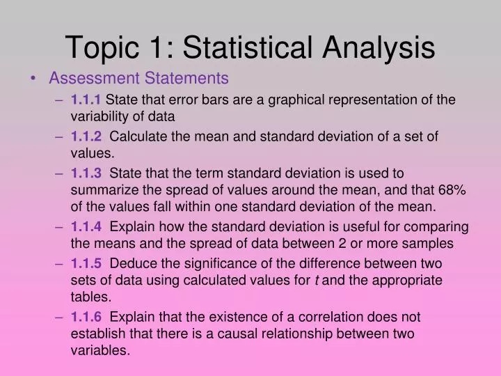
Topic 1: Statistical Analysis. Assessment Statements 1.1.1 State that error bars are a graphical representation of the variability of data 1.1.2 Calculate the mean and standard deviation of a set of values.

E N D
Topic 1: Statistical Analysis • Assessment Statements • 1.1.1 State that error bars are a graphical representation of the variability of data • 1.1.2 Calculate the mean and standard deviation of a set of values. • 1.1.3 State that the term standard deviation is used to summarize the spread of values around the mean, and that 68% of the values fall within one standard deviation of the mean. • 1.1.4 Explain how the standard deviation is useful for comparing the means and the spread of data between 2 or more samples • 1.1.5 Deduce the significance of the difference between two sets of data using calculated values for t and the appropriate tables. • 1.1.6 Explain that the existence of a correlation does not establish that there is a causal relationship between two variables.
Why use statistics? • In science, we are always making observations about the world around us. • Many times these observations result in the collection of measurable, quantitative data. • Using this data, we can ask questions based upon some of these observations and try to answer those questions.
Essential Statistics Terms • Mean: the average of the data points • Range: the difference between the largest and smallest observed values in a data set (the measure of the spread of the data) • Standard Deviation: a measure of how the individual observations of a data set are dispersed or spread out around the mean • Error bars: Graphical representation of the variability of data
Standard Deviation • Standard deviation is used to summarize the spread of values around the mean and to compare the means of data between two or more samples. • In a normal distribution, about 68% of all values lie within ±1 standard deviation of the mean. 95% will lie within ±2 standard deviations of the mean. • This normal distribution will form a bell curve • The shape of the curve tells us how close all of the data points are to the mean.
Calculating Standard Deviation • We can use the formula to solve for standard deviation… Σ(xi - (Σx)2 Sx = n n - 1 Example data: Ward pg.5 For calculator help, go to http://www.heinemann.co.uk/hotlinks ,enter code 4242p and click weblink 1.4a or 1.4b HOWEVER the easiest way to calculate…find an app online!!!!
D8 C1 Imagine we chose two children at random from two class rooms… … and compare their height …
D8 C1 … we find that one pupil is taller than the other WHY?
D8 C1 There is a significant difference between the two groups, so pupils in C1 are taller than pupils in D8 REASON 1: YEAR 7 YEAR 11
D8 C1 Sammy HAGRID (Year 9) (Year 9) By chance, we picked a short pupil from D8 and a tall one from C1 REASON 2:
How do we decide which reason is most likely? MEASURE MORE STUDENTS!!!
D8 C1 If there is a significant difference between the two groups… … the average or mean height of the two groups should be very… … DIFFERENT
D8 C1 If there is no significant difference between the two groups… … the average or mean height of the two groups should be very… … SIMILAR
Living things normally show a lot of variation, so… Remember:
C1 Sample D8 Sample Average height = 168 cm Average height = 162 cm It is VERY unlikely that the mean height of our two samples will be exactly the same Is the difference in average height of the samples large enough to be significant?
16 16 C1 Sample 14 14 12 12 10 10 Frequency Frequency 8 8 6 6 4 4 2 2 180-189 160-169 140-149 140-149 160-169 170-179 150-159 170-179 150-159 Height (cm) D8 Sample 180-189 Height (cm) We can analyse the spread of the heights of the students in the samples by drawing histograms Here, the ranges of the two samples have a small overlap, so… … the difference between the means of the two samples IS probably significant.
16 16 C1 Sample 14 14 12 12 10 10 Frequency Frequency 8 8 6 6 4 4 2 2 180-189 160-169 140-149 140-149 160-169 170-179 150-159 170-179 150-159 Height (cm) D8 Sample 180-189 Height (cm) Here, the ranges of the two samples have a large overlap, so… … the difference between the two samples may NOT be significant. The difference in means is possibly due to random sampling error
You can calculate standard deviation using the formula: (Σxi)2 Where: Sx is the standard deviation of sample Σ stands for ‘sum of’ xi stands for the individual measurements in the sample n is the number of individuals in the sample Σ(xi - Sx = n n - 1 To decide if there is a significant difference between two samples we must compare the mean height for each sample… … and the spread of heights in each sample. Statisticians calculate the standard deviation of a sample as a measure of the spread of a sample
MODE (CASIO fx-85MS) 2 SHIFT CLR 1 (Scl) = 2 3 1 DT 5 DT DT 4 3 (M+ Button) It is much easier to use the statistics functions on a scientific calculator! e.g. for data 25, 34, 13 Set calculator on statistics mode Clear statistics memory Enter data
( x ) AC SHIFT S-VAR (2 Button) 1 = AC SHIFT S-VAR 3 (xσn-1) = Calculate the mean 24 Calculate the standard deviation 10.5357
( x1– x2 ) Where: x1 is the mean of sample 1 s1 is the standard deviation of sample 1 n1 is the number of individuals in sample 1 x2 is the mean of sample 2 s2 is the standard deviation of sample 2 n2 is the number of individuals in sample 2 t = (s1)2 (s2)2 + n1 n2 Student’s t-test The Student’s t-test compares the averages and standard deviations of two samples to see if there is a significant difference between them. We start by calculating a number, t t can be calculated using the equation:
C1: x1 = D8: x2 = x2 – x1 = 168.27 – 161.60 = Worked Example: Random samples were taken of pupils in C1 and D8 Their recorded heights are shown below… Step 1: Work out the mean height for each sample 161.60 168.27 Step 2: Work out the difference in means 6.67
D8: C1: (s2)2 (s1)2 = = n2 n1 Step 3: Work out the standard deviation for each sample C1: s1 = 10.86 D8: s2 = 11.74 Step 4: Calculate s2/n for each sample 10.862÷ 15 = 7.86 11.742÷ 15 = 9.19
Step 5: Calculate (s2)2 (s2)2 (s1)2 (s1)2 (s1)2 = = (7.86 + 9.19) = + + + n2 n2 n1 n1 n1 (s2)2 n2 t = 6.67 = 4.13 x2 – x1 4.13 Step 6: Calculate t (Step 2 divided by Step 5) 1.62
Step 7: Work out the number of degrees of freedom d.f. = n1 + n2 – 2 = 15 + 15 – 2 = 28 Step 8: Find the critical value of t for the relevant number of degrees of freedom Use the 95% (p=0.05) confidence limit Critical value = 2.048 Our calculated value of t is below the critical value for 28d.f., therefore, there is no significant difference between the height of students in samples from C1 and D8
Do not worry if you do not understand how or why the test works Follow the instructions CAREFULLY You will NOT need to remember how to do this for your exam