Governing Equations II

1. Governing Equations II by Nils Wedi (room 007; ext. 2657) Thanks to Piotr Smolarkiewicz

2. Introduction • Continue to review and compare a few distinct modelling approaches for atmospheric and oceanic flows • Highlight the modelling assumptions, advantages and disadvantages inherent in the different modelling approaches

3. Dry “dynamical core” equations √ • Shallow water equations • Isopycnic/isentropic equations • Compressible Euler equations • Incompressible Euler equations • Boussinesq-type approximations • Anelastic equations • Compressible vs. Anelastic • Primitive equations (GovEq III) • Pressure or mass-based coordinate equations including equations used in IFS at ECMWF (GovEq III) √

4. Euler equations for isentropic inviscid motion

5. Euler equations for isentropic inviscid motion Speed of sound (in dry air 15ºC dry air ~ 340m/s)

6. Reference and environmental profiles Distinguish between • (only vertically varying) static reference or basic state profile(used to facilitate comprehension of the full equations) • Environmental or balanced state profile(used in general procedures to stabilize or increase the accuracy of numerical integrations; satisfies all or a subset of the full equations, more recently attempts to have a locally reconstructed hydrostatic balanced state or use a previous time step as the balanced state

7. The use of reference and environmental/balanced profiles • For reasons of numerical accuracy and/or stability an environmental/balanced state is often subtracted from the governing equations Clark and Farley (1984) 

8. *NOT* approximated Euler perturbation equations eg. Durran (1999) using:

9. Incompressible Euler equations eg. Durran (1999); Casulli and Cheng (1992); Casulli (1998);

10. Example of simulation with sharp density gradient Animation: "two-layer" simulation of a critical flow past a gentle mountain Compare to shallow water: reduced domain simulation with H prescribed by an explicit shallow water model

11. Two-layer t=0.15

12. Shallow water t=0.15

13. Two-layer t=0.5

14. Shallow water t=0.5

15. Classical Boussinesq approximation eg. Durran (1999)

16. Projection method Subject to boundary conditions !!!

17. Integrability condition With boundary condition:

18. Solution Ap = f Due to the discretization in space a banded matrix A arises with size (N x L)2 N=number of gridpoints, L=number of levels Classical schemes include Gauss-elimination for small problems, iterative methods such as Gauss-Seidel and over-relaxation methods. Most commonly used techniques for the iterative solution of sparse linear-algebraic systems that arise in fluid dynamics are the preconditioned conjugate gradient method, e.g. GMRES, and the multigrid method (Durran,1999). More recently, direct methods are proposed based on matrix-compression techniques (e.g. Martinsson,2009)

19. Importance of the Boussinesq linearization in the momentum equation Two layer flow animation with density ratio 1:1000 Equivalent to air-water Incompressible Euler two-layer fluid flow past obstacle Incompressible Boussinesq two-layer fluid flow past obstacle Two layer flow animation with density ratio 297:300 Equivalent to moist air [~ 17g/kg] - dry air Incompressible Euler two-layer fluid flow past obstacle Incompressible Boussinesq two-layer fluid flow past obstacle

20. Anelastic approximation Batchelor (1953); Ogura and Philipps (1962); Wilhelmson and Ogura (1972); Lipps and Hemler (1982); Bacmeister and Schoeberl (1989); Durran (1989); Bannon (1996);

21. Anelastic approximation Lipps and Hemler (1982);

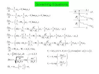
22. Numerical Approximation Compact conservation-law form: Lagrangian Form: 

23. Numerical Approximation with LE, flux-form Eulerian or Semi-Lagrangian formulation using MPDATA advection schemes Smolarkiewicz and Margolin (JCP, 1998)  with Prusa and Smolarkiewicz (JCP, 2003) specified and/or periodic boundaries

24. Importance of implementation detail? Example of translating oscillator (Smolarkiewicz, 2005): time

25. Example ”Naive” centered-in-space-and-time discretization: Non-oscillatory forward in time (NFT) discretization: paraphrase of so called “Strang splitting”, Smolarkiewicz and Margolin (1993)

26. Compressible Euler equations Davies et al. (2003)

27. Compressible Euler equations

28. Compressible vs. anelastic Davies et. al. (2003) Lipps & Hemler approximation Hydrostatic

29. Compressible vs. anelastic

30. Compressible vs. anelastic • Normal mode analysis done on linearized equations noting distortion of Rossby modes if equations are (sound-)filtered • Differences found with respect to deep gravity modes between different equation sets. Conclusions on gravity modes are subject to simplifications made on boundaries, shear/non-shear effects, assumed reference state, increased importance of the neglected non-linear effects. • The Anelastic/Boussinesq simplification in the momentum equation (not when pseudo-incompressible) simplifies baroclinic production of vorticity, i.e. possible steepening effect of vortices missing (see also §10.4 and Fig. 10.8 in Dutton (1967))

31. Compressible vs. anelastic • Recent scale analysis suggests the validity of anelastic approximations for weakly compressible atmospheres, low Mach number flows and realistic atmospheric stratifications (Δ 30K) (Klein et al., 2010), well beyond previous estimates! • Recently,Arakawa and Konor (2009) combined the hydrostatic and anelastic equations into a quasi-hydrostatic system potentially suitable for cloud-resolving simulations.