Understanding Differential Equations: Methods and Solutions

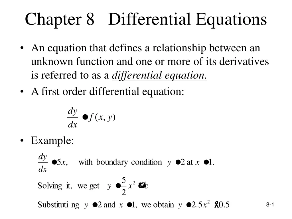
1. Chapter 8 Differential Equations • An equation that defines a relationship between an unknown function and one or more of its derivatives is referred to as a differential equation. • A first order differential equation: • Example:

2. Example: • A second-order differential equation: • Example:

3. Taylor Series Expansion • Fundamental case, the first-order ordinary differential equation: Integrate both sides • The solution based on Taylor series expansion:

4. Example : First-order Differential Equation Given the following differential equation: The higher-order derivatives:

5. The final solution:

6. Table: Taylor Series Solution

8. General Case • The general form of the first-order ordinary differential equation: • The solution based on Taylor series expansion:

9. Euler’s Method • Only the term with the first derivative is used: • This method is sometimes referred to as the one-step Euler’s method, since it is performed one step at a time.

10. Example: One-step Euler’s Method • Consider the differential equation: • For x =1.1 Therefore, at x=1.1, y=1.44133 (true value).

12. Errors with Euler`s Method • Local error: over one step size. Global error: cumulative over the range of the solution. • The error  using Euler`s method can be approximated using the second term of the Taylor series expansion as • If the range is divided into n increments, then the error at the end of range for x would be n.

13. Example: Analysis of Errors

14. Table: Local and Global Errors with a Step Size of 0.1.

15. Table: Local and Global Errors with a Step Size of 0.05.

16. Table: Local and Global Errors with a Step Size of 0.05 (continued).

17. Table: Local and Global Errors with a Step Size of 0.02.

18. Modified Euler’s Method • Use an average slope, rather than the slope at the start of the interval : • Evaluate the slope at the start of the interval • Estimate the value of the dependent variable y at the end of the interval using the Euler’s metod. • Evaluate the slope at the end of the interval. • Find the average slope using the slopes in a and c. • Compute a revised value of the dependent variable y at the end of the interval using the average slope of step d with Euler’s method.

19. Example : Modified Euler’s Method

21. Second-order Runge-Kutta Methods • The modified Euler’s method is a case of the second-order Runge-Kutta methods. It can be expressed as

22. The computations according to Euler’s method: • Evaluate the slope at the start of an interval, that is, at (xi,yi) . • Evaluate the slope at the end of the interval (xi+1,yi+1) : • Evaluate yi+1 using the average slope S1 of and S2 :

23. Third-order Runge-Kutta Methods • The following is an example of the third-order Runge-Kutta methods :

24. The computational steps for the third-order method: • Evaluate the slope at (xi,yi). • Evaluate a second slope S2 estimate at the mid-point in of the step as • Evaluate a third slope S3 as • Estimate the quantity of interest yi+1 as

25. Fourth-order Runge-Kutta Methods • Compute the slope S1 at (xi,yi). • Estimate y at the mid-point of the interval. • Estimate the slope S2 at mid-interval. • Revise the estimate of y at mid-interval

26. Compute a revised estimate of the slope S3 at mid-interval. • Estimate y at the end of the interval. • Estimate the slope S4 at the end of the interval • Estimate yi+1again.

27. Predictor-Corrector Methods • Unless the step sizes are small, Euler’s method and Runge-Kutta may not yield precise solutions. • The Predictor-Corrector Methods iterate several times over the same interval until the solution converges to within an acceptable tolerance. • Two parts: predictor part and corrector part.

28. Euler-trapezoidal Method • Euler’s method is the predictor algorithm. • The trapezoidal rule is the corrector equation. • Eluer formula (predictor): • Trapezoidal rule (corrector): The corrector equation can be applied as many times as necessary to get convergence.

29. Example 8-6: Euler-trapezoidal Mehtod

33. Milne-Simpson Method • Milne’s equation is the predictor euqation. • The Simpson’s rule is the corrector formula. • Milne’s equation (predictor): For the two initial sampling points, a one-step method such as Euler’s equation can be used. • Simpsos’s rule (corrector):

34. Example 8-7: Milne-Simpson Mehtod Assume that we have the following values, obtained from the Euler-trapezoidal method in Example 8-6.

36. The computations for x=1.3 are complete.

37. The Milne predictor equation for estimating y at x=1.4: The corrector formular:

39. Least-Squares Method • The procedure for deriving the least-squares function: • Assume the solution is an nth-order polynomial: • Use the boundary condition of the ordinary differential equation to evaluate one of (bo,b1,b2,…,bn). • Define the objective function:

40. Find the minimum of F with respect to the unknowns (b1,b2, b3,…,bn) , that is • The integrals in Step 4 are called the normal equations; the solution of the normal equations yields value of the unknowns (b1,b2, b3,…,bn).

41. Example 8-8: Least-squares Method • First, assume a linear model is used:

43. Table: A linear model for the least-squares method

44. Next, to improve the accuracy of estimates, a quadratic model is used:

47. Table: A quadratic model for the least-squares method

48. Galerkin Method • Example: Galerkin Method The same problem as Example 8-8. Use the quadratic approximating equation.

50. Table: Example for the Galerkin method