Download

1 / 27
270 likes | 299 Views
This study addresses the computation of reachability in uncertain graphs with distance constraints, focusing on approximating solutions with low computational cost. Various estimators and sampling approaches are explored, aiming to reduce variance and improve efficiency. Experimental results on synthetic and real datasets are presented.

E N D
Distance-Constraint Reachability Computation in Uncertain Graphs Ruoming Jin, Lin LiuKent State University Bolin Ding UIUC Haixun Wang MSRA
Why Uncertain Graphs? Increasing importance of graph/network data Social Network, Biological Network, Traffic/Transportation Network, Peer-to-Peer Network Probabilistic perspective gets more and more attention recently. Uncertainty is ubiquitous! Protein-Protein Interaction Networks Social Networks Probabilistic Trust/Influence Model False Positive > 45%
Uncertain Graph Model Edge Independence • Possible worlds (2#Edge) Existence Probability G1: G2: Weight of G2: Pr(G2) = 0.5 0.7 0.2 0.6 (1-0.5) * * * * (1-0.4) (1-0.9) (1-0.1) (1-0.3) = 0.0007938 * * * *
Distance-Constraint Reachability (DCR) Problem Given distance constraint d and two vertices s and t, • What is the probability that s can reach t within distance d? • A generalization of the two-terminal network reliability problem, which has no distance constraint. Target Source
Important Applications • Peer-to-Peer (P2P) Networks • Communication happens only when node distance is limited. • Social Networks • Trust/Influence can only be propagated only through small number of hops. • Traffic Networks • Travel distance (travel time) query • What is the probability that we can reach the airport within one hour?
Example: Exact Computation • d = 2, ? First Step: Enumerate all possible worlds (29), Pr(G1) Pr(G2) Pr(G3) Pr(G4) Second Step: Check for distance-constraint connectivity, … + Pr(G1) * 0 + Pr(G2) * 1 + Pr(G3) * 0 + Pr(G4) * 1 + … =
Approximating Distance-Constraint Reachability Computation • Hardness • Two-terminal network reliability is #P-Complete. • DCR is a generalization. • Our goal is to approximate through Sampling • Unbiased estimator • Minimal variance • Low computational cost
Direct Sampling Approach • Sampling Process • Sample n graphs • Sample each graph according to edge probability
Direct Sampling Approach (Cont’) • Estimator • Unbiased • Variance = 1, s reach t within d; = 0, otherwise. Indicator function
Path-Based Approach • Generate Path Set • Enumerate all paths from s to twith length ≤ d • Enumeration methods • E.g., DFS
Path-Based Approach (Cont’) • Path set • Exactly computed by Inclusion-Exclusion principle • Approximated by Monte-Carlo Algorithm by R. M. Karp and M. G. Luby ( ) • Unbiased • Variance
Divide-and-Conquer Methodology • Example +(s,a) -(s,a) -(s,b) +(s,b) -(a,t) +(a,t) … … … … … …
Divide and Conquer (Cont’) Summarize: • # of leaf nodes is smaller than 2|E| . • Each possible world exists only in one leaf node. • Reachability is the sum of the weights of blue nodes. • Leaf nodes form a nice sample space. all possible worlds Graphs having e1 Graphs not Having e1 s can reach t. s can not reach t.
How do we sample? Start from here • Unequal probability sampling • Hansen-Hurwitz (HH) estimator • Horvitz-Thomson (HT) estimator Pri: Sample Unit Weight; Sum of possible worlds’ probabilities in the node. qi: sampling probability, determined by properties of coins along the way. Sample Unit
Hansen-Hurwitz (HH) Estimator sample size = 1, blue node = 0, red node • Estimator • Unbiased • Variance Weight Sampling probability To minimize the variance above, we have :Pri = qi Pri = p(e1)*p(e2)*(1-p(e3))*… Pri: the leaf node weight qi: the sampling probability P(e1) 1-P(e1) p(e1) : 1 – p(e1) P(e2) 1-P(e2) 1-P(e4) P(e4) 1-P(e3) p(e2) : 1 – p(e2) P(e3) p(e3) : 1 – p(e3)
Horvitz-Thomson (HT) Estimator # of Unique sample units • Estimator • Unbiased • Variance • To minimize vairance, we find Pri = qi • Smaller variance than HH estimator
Recursive Estimator • Unbiased • Variance: n1 + n2 = n Sample the entire space n times Sample the sub-space n1 times Sample the sub-space n2 times We can not minimize the variance without knowing τ1 and τ2. Then what can we do?
Sample Allocation • We guess: What if • n1 = n*p(e) • n2 = n*(1-p(e))? • We find: Variance reduced! • HH Estimator: • HT Estimator:
Sample Allocation (Cont’) Sample size = n • Sampling Time Reduced!! Directly allocate samples n1=n*p(e1) n2=n*(1-p(e1)) n3=n1*p(e2) n4=n1*(1-p(e2)) Toss coin when sample size is small
Experimental Setup • Experiment setting • Goal: • Relative Error • Variance • Computational Time • System Specification • 2.0GHz Dual Core AMD Opteron CPU • 4.0GB RAM • Linux
Experimental Results • Synthetic datasets • Erdös-Rényi random graphs • Vertex#: 5000, edge density: 10, Sample size: 1000 • Categorized by extracted-subgraph size (#edge) • For each category, 1000 queries
Experimental Results • Real datasets • DBLP: 226,000 vertices, 1,400,000 edges • Yeast PPIN: 5499 vertices, 63796 edges • Fly PPIN: 7518 vertices, 51660 edges • Extracted subgraphs size: 20 ~ 50 edges
Conclusions • We first propose a novel s-t distance-constraint reachability problem in uncertain graphs. • One efficient exact computation algorithm is developed based on a divide-and-conquer scheme. • Compared with two classic reachability estimators, two significant unequal probability sampling estimatorsHansen-Hurwitz (HH) estimator and Horvitz-Thomson (HT) estimator. • Based on the enumeration tree framework, two recursive estimators Recursive HH, and Recursive HT are constructed to reduce estimation variance and time. • Experiments demonstrate the accuracy and efficiency of our estimators.
Thank you ! Questions?