Download

1 / 51
2.63k likes | 4.85k Views
Introduction to Simulink. Presentation Outline. What is Simulink? Basic operations with Simulink Examples Exercise. What is Simulink?. Simulink is an interactive tool for modeling, simulating and analyzing dynamic systems.

E N D
Presentation Outline • What is Simulink? • Basic operations with Simulink • Examples • Exercise
What is Simulink? • Simulink is an interactive tool for modeling, simulating and analyzing dynamic systems. • Simulink integrates seamlessly with MATLAB, providing immediate access to an extensive range of analysis and design tools. • Simulating a dynamic system is a two-step process with Simulink: • create a model of the system to be simulated using Simulink’s model editor (BLOCK DIAGRAM) • use Simulink to simulate the behavior of the system for a specified time span
Launch Simulink • First launch MATLAB. • To open Simulink, type simulink at the MATLAB command window or click on the Simulink icon on the MATLAB toolbar.
Simulink Block Libraries Simulink provides a library browser that allows you to select blocks from libraries of standard blocks: • Continuous - blocks that describe linear functions • Discrete - blocks that describe discrete-time components • Functions & Tables - general functions and table look-up operations • Math - blocks that describe general mathematics functions
Simulink Block Libraries • Nonlinear- blocks that describe nonlinear functions • Signal & systems - blocks that allow multiplexing, de-multiplexing, implement external input/output, pass data to other parts of the model, create subsystems and perform other functions • Sinks - blocks that display or write block output • Sources - blocks that generate signals • Blocksets and toolboxes - the extras block library of specialized blocks
Creating a New Model • Click the new-model icon in the upper left corner to start a new Simulink file • Select the Simulink icon to obtain elements of the model
Your Workspace Library of elements Model is created in this window Show/hide Library Browser
Block Diagram A Simulink block diagram is a pictorial model of a dynamic system. It consists of blocks interconnected by lines. Blocks represent elementary dynamical systems that Simulink knows how to simulate. A block comprises one or more of the following: • A set of inputs. • A set of states. • A set of outputs. To introduce blocks in your model, choose the block from the library, click on it and drag it in your model. Double clicking on the block will allow you to change the block parameters.
Model Execution Phase In this phase Simulink successively computes the states and the outputs of the system at intervals from the simulation start time to the stop time, using information provided by the model. Time steps - successive time points at which the states and the outputs are computed. Step size - the length of time between steps. It depends on the type of solver: • Fixed-step - a smaller step size produces a more accurate simulation but results in a longer execution time.
Model Execution Phase • Variable step - depending on the application, it can produce more accurate results without sacrificing execution speed. Parameters set up: Simulation > Simulationparameters … Simulink simulates a system when you choose start from the model editor’s simulation menu.
Example 1: a Simple Model • Build a Simulink model that solves the differential equation • Initial condition • First, sketch a simulation diagram of this mathematical model (equation) (3 min.)
x (0) = -1 1 x . 3sin(2t) (input) x(t) (output) x s integrator Simulation Diagram • Input is the forcing function 3sin(2t) • Output is the solution of the differential equation x(t) • Now build this model in Simulink
Select in Input Block Drag a Sine Wave block from the Sources library to the model window
Select an Operator Block Drag an Integrator block from the Continuous library to the model window
Select an Output Block Drag a Scope block from the Sinks library to the model window
Connect Blocks with Signals • Place your cursor on the output port (>) of the sine wave block • Drag from the sine wave output to the integrator input • Drag from the integrator output to the scope input Arrows indicate the direction of the signal flow.
Select Simulation Parameters Double-click on the Sine Wave block to set amplitude = 3 and freq = 2 This produces the desired input of 3sin(2t)
Select Simulation Parameters Double-click on the Integrator block to set initial condition = -1 This sets our IC x(0) = -1.
Run the Simulation In the model window, from the Simulation pull-down menu, select Start Double-click on the Scope to view the simulation results
Simulation Results To verify that this plot represents the solution to the problem, solve the equation analytically. The analytical result, matches the plot (the simulation result) exactly.
Example 2 • Build a Simulink model that solves the following differential equation • 2nd-order mass-spring-damper system • Zero ICs • Input f(t) is a step with magnitude 3 • Parameters: m = 0.25, c = 0.5, k = 1 • m->mass; c->damping factor; k->spring constant
k m f (t) x c Example 2
Create the Simulink Diagram • On the following slides: • The simulation diagram for solving the ODE is created step by step. • After each step, elements are added to the Simulink model. • Optional exercise: first, sketch the complete diagram (5 min.).
.. mx summing block Create the Block Diagram • First, solve for the term with highest-order derivative • Make the left-hand side of this equation the output of a summing block
Drag a Sum block from the Math library Double-click to change the block parameters to rectangular and + - -
.. .. mx x Create the Block Diagram • Add a gain (multiplier) block to eliminate the coefficient and produce the highest-derivative alone 1 m summing block
Drag a Gain block from the Math library The gain is 4 since 1/m = 4. Double-click to change the block parameters. Add a title.
summing block Create the Block Diagram • Add integrators to obtain the desired output variable
Drag Integrator blocks from the Continuous library ICs on the integrators are zero. Add a scope from the Sinks library. Connect output ports to input ports. Label the signals by double-clicking on the leader line.
summing block c k Create the Block Diagram • Connect to the integrated signals with gain blocks to create the terms on the right-hand side of the equation
Drag new Gain blocks from the Math library To flip the gain block, select it and choose Flip Block in the Format pull-down menu or double-clock on it. c = 0.5 • Double-click on gain blocks to set parameters • Connect from the gain block input backwards up to the branch point. • Re-title the gain blocks. K = 1.0
Complete the Model • Bring all the signals and inputs to the summing block. • Check signs on the summer. f(t) input + x(t) output - - c k
Double-click on Step block to set parameters. For a step input of magnitude 3, set Final value to 3
Results Underdamped response. Overshoot of 0.5. Final value of 3. Is this expected?
Checking Results • Standard form • Natural frequency • Damping ratio • Static gain
Checking Results • Damping ratio of 0.5 is less than 1: • Expect the system to be underdamped. • Expect to see overshoot. • Static gain is 1: • Expect output magnitude to equal input magnitude. • Input has magnitude 3, so does output. Simulation results conform to expectations
Saving to Workspace Drag the To Workspace block from the Sink library
Saving to Workspace Double click on the To Workspace block to change the parameters. Check on MATLAB workspace if the variable is there. Example: plot (tout, x); y = sqrt (x )
Inserting a S-Function Drag a S-Function block from the Functions & Tables library
Inserting a S-Function Double click on the S-Function block to change the S-Function name and include additional parameters. Use the template that comes with Simulink. Change the template based on your project.
Inserting a S-Function • Type sfundemos at the MATLAB command line. • Double click on M-files • Double click on M-file S-Function Template • Save the file in another folder and with another name • Change the function name: • function [sys,x0,str,ts]=sfungains(t,x,u,flag)
Inserting a S-Function • Change the S-Function size parameters: • sizes = simsizes; • sizes.NumContStates = 0; • sizes.NumDiscStates = 0; • sizes.NumOutputs = 2; • sizes.NumInputs = 0; • sizes.DirFeedthrough = 0; • sizes.NumSampleTimes = 1; % at least one sampletime is • needed • sys = simsizes(sizes);
Inserting a S-Function • Edit the mdlOutputs m-function in accordance to your project: • function sys=mdlOutputs(t,x,u) • K1 = 50; • K2 = 20; • sys = [K1 K2];
Inserting a S-Function Drag a Demux block from the Signals & Systems library
Inserting a S-Function Drag Display blocks from the Sink library Run your project
K3 + u y + + K1 K4 _ + K2 K5 Exercise Given the following block diagram: