Download
1 / 51
510 likes | 610 Views
Wiggler modeling Double-helix like option. Simona Bettoni and Remo Maccaferri, CERN. Outline. Introduction The model 2D (Poisson) 3D (Opera Vector Fields-Tosca) The analysis tools Field uniformity Multipoles (on axis and trajectory) Tracking studies The integrals of motion cancellation

E N D
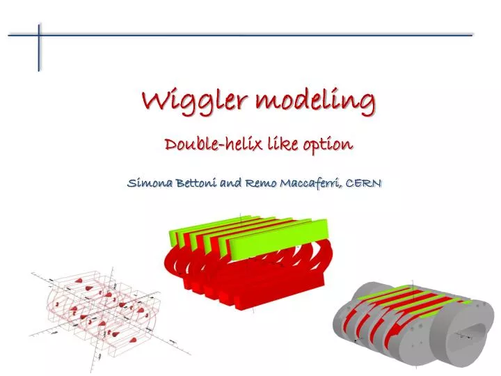
Wiggler modelingDouble-helix like option Simona Bettoni and Remo Maccaferri, CERN
Outline • Introduction • The model • 2D (Poisson) • 3D (Opera Vector Fields-Tosca) • The analysis tools • Field uniformity • Multipoles (on axis and trajectory) • Tracking studies • The integrals of motion cancellation • Possible options • The final proposal • The prototype analysis • Conclusions
Wigglers/undulators model Large gap & long period mid-plane Small gap & short period
2D design (proposed by R. Maccaferri) • Advantages: • Save quantity of conductor • Small forces on the heads (curved part) BEAM
The 3D model (conductors) Conductors generated using a Matlab script • Conductors grouped to minimize the running time • Parameters the script: • Wire geometry (l_h, l_v, l_trasv) • Winding “shape” (n_layers, crossing positions)
The analysis tools • Tracking analysis: • Single passage: ready/done • Multipassage: to be implemented • Field uniformity: ready/done • Multipolar analysis: • Around the axis: ready /done • Around the reference trajectory: ready x and x’ at the exit of the wiggler
Prototype analysis z x y
Field distribution on the conductors BMod (Gauss) • Maximum field and forces (PMAX ~32 MPa) on the straight part • Manufacture: well below the limit of the maximum P for Nb3Sn • Simulation: quick to optimize the margin (2D)
The 2D/3D comparison 1.9260 T 2D (Poisson) -2.1080 T 1.9448 T 3D (Tosca) -2.1258 T
Tracking studies Trajectory x-shift at the entrance = ± 3 cm z x y
Tracking studies: the exit position Subtracting the linear part
Integrals of motion = 0 for anti-symmetry 1st integral 2nd integral Offset of the oscillation axis CLIC case: even number of poles (anti-symmetric) No offset of the oscillation axis
Integrals of motion: the starting point = 0 for anti-symmetry 1st integral 2nd integral (cm)
Lowering the 2nd integral: what do we have to do? To save time we can do tracking studies in 2D up to a precision of the order of the difference in the trajectory corresponding to the 2D/3D one (~25 mm) and only after refine in 3D.
Lowering the 2nd integral: how can we do? → Highly saturated → → • What we can use: • End of the yoke length/height • Height of the yoke • Terminal pole height (|B| > 5 T) • Effectiveness of the conductors
The multipoles of the option 1 Starting configuration (CLICWiggler_7) Modified (option 1) (CLICWiggler_8)
Option 1 vs option 2 • The “advantage” of the option 2: • Perfect cancellation of the 2nd integral • Field well confined in the yoke • Possibility to use only one IN and one OUT (prototype) • The “disadvantage” of the option 2: • Comments? • The “advantage” of the option 1: • Quick to be done • The “disadvantage” of the option 1: • Not perfect cancellation of the 2nd integral • Field not completely confined in the yoke • Multipoles get worse → start → → → end → 1st layers (~1/3 A*spire equivalent) All the rest
Lowering the 2nd integral: option 2 (3D) If only one IN and one OUT → discrete tuning in the prototype model
Tracking studies (optimized configuration) Not optimized Optimized
Working point: Nb3Sn & NbTi Wire diameter (insulated) = 1 mm Wire diameter (bare) = 0.8 mm Non-Cu fraction = 0.53 Cu/SC ratio = 1 * Nb3Sn NbTi Nb3Sn NbTi *MANUFACTURE AND TEST OF A SMALL CERAMIC-INSULATED Nb3Sn SPLIT SOLENOID, B. Bordini et al., EPAC’08 Proceedings.
Possible configurations Possible to increase the peak field of 0.5 T using holmium
Conclusions • A novel design for the CLIC damping ring has been analyzed (2D & 3D) • Advantages: • Less quantity of conductor needed • Small forces on the heads • Analysis on the prototype: • Maximum force • Multipolar analysis • Tracking studies • Zeroing the integrals of motion • Future plans • Optimization of the complete wiggler model (work in progress): • Best working point definition • Modeling of the long wiggler • 2nd integral optimization for the long model • Same analysis tools applied to the prototype model (forces, multipoles axis/trajectory, tracking) • Minimization of the integrated multipoles
Longitudinal field (By = f(y), several x) • Scan varying the entering position in horizontal, variation in vertical: • Dz = 0.1 mm for x-range = ±1 cm • Dz = 2 mm for x-range = ±2 cm
Horizontal transverse field (Bx = f(y), several x) • Scan varying the entering position in horizontal, variation in vertical: • Dz = 0.1 mm for x-range = ±1 cm • Dz = 2 mm for x-range = ±2 cm
Controlling the y-shift: cancel the residuals W1 W2 W3 W4 W1 W2 W3 W4 2 mm in 10 cm -> 20*2 = 40 mm in 2 m
Controlling the x-shift: cancel the residuals (during the operation) To be evaluated the effect of the kicks given by the quadrupoles W1 W2 … Entering at x = 0 cm Entering at x = -DxMAX/2 • Entering at x = +DxMAX/2 (opposite I wiggler … positron used for trick)
Tracking at x-range = ±3 cm: exit position Subctracting the linear part
Long wiggler modeling • Problem: very long running time (3D) because of the large number of conductors in the model • Solution: • Build 2D models increasing number of periods until the field distribution of the first two poles from the center give the same field distribution (Np) • Build 3D model with a number of poles Np • “Build” the magnetic map from this


![[READ DOWNLOAD] DNA Demystified: Unravelling the Double Helix](https://cdn7.slideserve.com/12657144/read-download-dna-demystified-unravelling-dt.jpg)