Download
1 / 11
110 likes | 206 Views
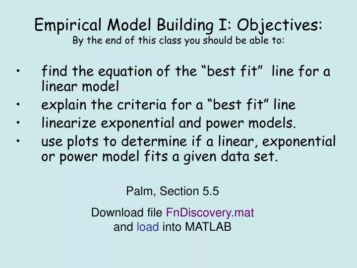
Empirical Model Building I: Objectives: By the end of this class you should be able to:. find the equation of the “best fit” line for a linear model explain the criteria for a “best fit” line linearize exponential and power models.

E N D
Empirical Model Building I: Objectives:By the end of this class you should be able to: • find the equation of the “best fit” line for a linear model • explain the criteria for a “best fit” line • linearize exponential and power models. • use plots to determine if a linear, exponential or power model fits a given data set. Palm, Section 5.5 Download file FnDiscovery.mat and load into MATLAB
Review Exercise (pairs) The compressive strength of samples of a specific type of cement can be modeled by a normal distribution with a mean of 6000 kilograms per square centimeter and a standard deviation of 100 kilograms per square centimeter • What is the variance of this compressive strength? • What percent of a batch of cement samples is expected to be greater than 5800 kg/cm2? Adapted from: Montgomery, Runger and Hubele, Engineering Statistics, 2nd Ed., Wiley (2001)
Expected Proportions for known mean Percentage of observations in the given range 68 % 1s 95.5 % 99.7% 2s 3s
Modeling Spring Lengthening What type of model (equation) would you use to represent the data below? Why?
Capacitor Discharge DataPlot this data.Can you fit a linear model to it?
Three Basic Two-parameter Models(colored equations down on a blank paper) • Linear • Power • Exponential or
Remember basic Log/ln rules • Multiplication: log(ab) = log(a) + log(b) or ln(ab) = ln(a) + ln(b) • Powers: log(am) = m log(a) or ln(am) = m ln(a) For the power and exponential models you wrote down :Take the log of both sides and simplify
Log transformations: >> log(x) the natural log of x (i.e., ln(x)) >> log10(x) the base 10 log of x This pattern is typical for many programs Also remember: >> semilogy(x,y, ...) creates a plot with a log scale on the y axis >> loglog(x,y, ...) creates a plot with log scales on both axes A few notes on MatLAB commands
Function Discovery: 2-parameter models(Try to find a plot that makes the data look linear)
Exercise: Determine the likely model form for: 1. Deflection of a cantilever beam (F, d) 2. x1 vs. y1 3. x2 vs y2 Data vectors Available • On handout • In MATLAB data file FnDiscovery.mat