Download
1 / 23
400 likes | 810 Views
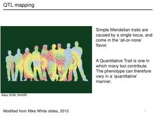
QTL mapping. Simple Mendelian traits are caused by a single locus, and come in the ‘ all-or-none ’ flavor. A Quantitative Trait is one in which many loci contribute. The phenotype can therefore vary in a ‘ quantitative ’ manner. Ades 2008, NHGRI. Modified from Mike White slides, 2010.

E N D
QTL mapping Simple Mendelian traits are caused by a single locus, and come in the ‘all-or-none’ flavor. A Quantitative Trait is one in which many loci contribute. The phenotype can therefore vary in a ‘quantitative’ manner. Ades 2008, NHGRI Modified from Mike White slides, 2010
Goals of QTL mapping • To identify the loci that contribute to phenotypic variation • Cross two parents with extreme phenotypes • Score the progeny for the phenotype • Genotype the progeny at markers across the genome • Associate the observed phenotypic variation with the underlying genetic variation • Ultimate goal: identify causal polymorphisms that explain the phenotypic variation Ades 2008, NHGRI Modified from Mike White slides, 2010
Backcross Phenotype: Drug tolerance 80% 20% viability Usually have at least 100 individuals Broman and Sen 2009
Intercross Phenotype: Drug tolerance 80% 20% viability Broman and Sen 2009
Backcross vs. Intercross • An intercross recovers all three possible genotypes (AA, BB, AB). This allows detection of dominance with both alleles and provides estimates of the degree of dominance. • A backcross has more power to detect QTL with fewer individuals. • A backcross may be the only possible scheme when crossing two different species.
Genetic map: specific markersspaced across the genome • Markers can be: • SNPs at particular loci • Variable-length repeats • e.g. ALU repeats • ALL polymorphisms • (if have whole genomes) Ideally, markers should be spaced every 10-20 cM and span the whole genome
Statistical framework • Missing Data Problem • Use marker data to infer intervening genotypes • 2. Model Selection Problem • How do the QTL across the genome combine with the covariates to generate the phenotype? Broman and Sen 2009
Marker regression: simple T-test (or ANOVA) at each marker Marker 1: no QTL Marker 2: significant QTL (population means are different)
Marker regression Advantages: • Simple test – standard T-test/ANOVA • Covariates (e.g. Gender, Environment) are to incorporate • No genetic map necessary, since test is done separately on each marker Disadvantages: • Any individuals with missing marker data must be omitted from analysis • Does not effectively consider positions between markers • Does not test for genetic interactions (e.g. epistasis) • The effect size of the QTL (i.e. power to detect QTL) is reduced by incomplete • linkage to the marker • Difficult to pinpoint QTL position, since only the marker positions are considered
Interval mapping • Lander and Botstein 1989 • In addition to examining phenotype-genotype associations at markers, look for associations between makers by inferring the genotype A A A A Q • The methods for calculating genotype probabilities between markers typically use hidden Markov models to account for additional factors, such as genotyping errors
Interval mapping Broman and Sen 2009
Interval mapping – maximum likelihood 1. Calculate genotype probabilities at intervening locations for every individual A A A A • At a marker, calculate the conditional probability that an individual is in one of the two QTL genotype groups (AA or AB) given their phenotype and the current estimates of µAA(s-1)and µAB(s-1)(Expectation Step) • Calculate new estimates of µAA(s)and µAB(s),by combining the genotype probabilities of each individual with their phenotypic values (Maximization Step) • Repeat until the estimates of µAA(s-1),µAA(s)and µAB(s-1),µAB(s) converge.
Interval mapping Advantages: • Takes account of missing genotype information – all individuals are included • Can scan for QTL at locations in between markers • QTL effects are better estimated Disadvantages: • More computation time required • Still only a single-QTL model – cannot separate linked QTL or examine for interactions among QTL
LOD scores • Measure of the strength of evidence for the presence of a QTL • at each marker location LOD(λ) = log10 likelihood ratio comparing the hypothesis of a QTL at position λ versus that of no QTL } { Pr(y|QTL at λ, µAAλ,µABλ,σλ) log10 Pr(y|no QTL, µ,σ) LOD 3 means that the TOP model is 103 times more likely than the BOTTOM model Phenotype
LOD curves How do you know which peaks are really significant?
LOD threshold • Consider the null hypothesis that there are no QTLs genome-wide one location genome-wide Randomize the phenotype labels on the relative to the genotypes Conduct interval mapping and determine what the maximum LOD score is genome-wide Repeat a large number of times (1000-10,000) to generate a null distribution of maximum LOD scores Broman and Sen 2009
Leoine Moyle, Indiana University “Dissecting Speciation via the Genetics of Isolation and Adaptation” Genetics Colloquium Wednesday, March 14 3:30 pm Biotech Center Auditorium Room 1111
LOD threshold • 1000 permutations • 10% False Discovery Rate = LOD 3.19 • (means that at this LOD cutoff 10% of peaks could be random chance) • 5% FDR = LOD 3.52 • Boundary of the peak is often taken as points that cross (Max LOD – 1.5) (or - 1.8 for an intercross)
LOD curves – Marker regression vs. interval mapping IM MR • With complete marker genotype information, marker regression would give the same results as interval mapping
Other mapping methods • Methods discussed assume single QTL models • Multiple QTLs on a chromosome are not estimated correctly • Cannot detect a QTL whose effect is dependent on the genotype at a second QTL (epistasis) Can also apply other Models • Two-dimensional two-QTL scans • Consider all pairs of markers across the genome • Multiple QTL Models • Jointly estimate all sets of QTL, interactions, and covariates in a single, coherent model • Focuses on the model selection problem of QTL mapping
From QTL to candidate genes • F2 mapping results in large loci associated with the phenotype • Mapping a QTL that explains 5% of the phenotypic variance in 300 F2 animals will yield a region approximately 40 cM in size (800 genes in mice!) • 2050 mouse and 700 rat QTL have been mapped (reviewed in Flint et al. 2005) • ~20 underlying genes have been identified • Strategies for getting to causal loci: • Generate additional recombinants to fine map QTL • Effect sizes of QTL can be overestimated • Often one large QTL is composed of manly tightly linked QTL of small effect • Identify candidate genes from known mutants, tissue-specific expression, etc. • Identify candidate genes through comparison to association mapping studies or population genomics studies • Are the results repeatable across environments? • Association mapping and population genomics approaches only identify alleles with large effect sizes