Download
1 / 21
680 likes | 1.91k Views
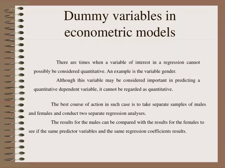
Dummy variables in econometric models. There are times when a variable of interest in a regression cannot possibly be considered quantitative. An example is the variable gender.

E N D
Dummy variables in econometric models There are times when a variable of interest in a regression cannot possibly be considered quantitative. An example is the variable gender. Although this variable may be considered important in predicting a quantitative dependent variable, it cannot be regarded as quantitative. The best course of action in such case is to take separate samples of males and females and conduct two separate regression analyses. The results for the males can be compared with the results for the females to see if the same predictor variables and the same regression coefficients results.
If a large sample size is not possible, a dummy variable can be employed to introduce qualitative variable into the analysis. A DUMMY VARIABLE IN A REGRESSION ANALYSIS IS A QUALITATIVE OR CATEGORICAL VARIABLE THAT IS USED AS A PREDICTOR VARIABLE.
For example, a male could be designated with the code 0 and the female could be coded as 1. Each person sampled could then be measured as either a 0 or a 1 for the variable gender, and this variable, along with the quantitative variables for the persons, could be entered into a multiple regression program and analyzed.
Example 1 Returning to real-estate developer, we noticed that all the houses in the population were from three neighborhoods, A, B, and C.
Using these data, we can construct the necessary dummy variables and determine whether they contribute significantly to the prediction of home size (Y). One way to code neighborhoods would be to define:
However, this type of coding has many problems. First, because 0 < 1< 2, the codes imply that neighborhood A is smaller then neighborhood B, which is smaller then neighborhood C. A better procedure is to use the necessary number of dummy variables to represent the neighborhood.
To represent the three neighborhoods, we use two dummy variables, by letting
What happened to neighborhood C? It is not necessary to develop a third dummy variable. IT IS VERY IMPORTANT THAT YOU NOT INCLUDE IT!! If you attempted to use three such dummy variables in your model, you would receive a message in your computer output informing you that no solution exists for this model.
Why? One predictor variable is a linear combination (including a constant term) of one or more other predictors, then mathematically no solution exists for the least squares coefficients. To arrive at a usable equation, any such predictor variable must not be included. We don’t lose any information – this excluded category is the reference system. The coefficients are the measure of the categories included in comparison to this one excluded.
The results of LINEST The regression equation explains 92% of the variability of home sizes
· If family income increases 1000$ the average home size will increase about 0,082 hundred of square feet (holding family size constant) · If family size increases 1 person the average home size will increase about 3,27 hundred of square feet (holding family income constant)
· The houses located in neighborhood A are 1,613 hundred of square feet bigger then houses from neighborhood C. · The houses located in neighborhood B are 0,9 hundred of square feet smaller then houses from neighborhood C.
Example 2 Joanne Herr, an analyst for the Best Foods grocery chain, wanted to know whether three stores have the same average dollar amount per purchase or not. Stores can be thought of a single qualitative variable set at 3 levels – A, B, and C.
A model can be set up to predict the dollar amount per purchase: where Y^- expected dollar amount per purchase
The data The variables X1 and X2 are dummy variables representing purchases in store A or B, respectively. Note that the three levels of the qualitative variable have been described with only two variables.
The regression equation explains 64% of the variability of average dollar amount per purchase.
· the average dollar amount per purchase is for store A is 10,01$ higher comparing with store C · the average dollar amount per purchase is for store B is 9,42$ higher comparing with store C always compare to the excluded category!!
Store A Store B Store C