Download
1 / 12
120 likes | 147 Views
This slide show provides a detailed step-by-step view of a simple peak-fit analysis process. It includes defining data points, setting baseline endpoints, selecting baseline shapes, modifying Gaussian:Lorentzian ratios, defining peaks using boxes, starting the peak fit, adjusting parameters via the Peak-Fit Table, and assessing fit quality via residuals.

E N D
Peak-Fitting • This slide show presents a Step-by-Step view of a simple peak-fit • We first define the number of “data” points to define the end points • Then we use the mouse cursor to define the baseline end points • Next we choose one of 3 different baseline shapes (use the icons) • If desired we can change the “Default Fit Parameters” that define the Gaussian:Lorentzian ratios (only the Gaussian % is shown) • Now we draw a series of “boxes” one by one to define the peaks (we can use the “Add Peak-Fit Peak” shortcut icon or the menu item) • Then we start the peak-fit by selecting the “Start Peak-Fit” icon. • To change or control any of the peak-fit parameters we need to open the “Peak-Fit Table” • We can check on the goodness of the fit by looking at a “Residual”