Download

1 / 21
220 likes | 432 Views
Transformations to Achieve Linearity. Created by Mr. Hanson. Objectives. Course Level Expectations CLE 3136.2.3 Explore bivariate data Check for Understanding (Formative/Summative Assessment)

E N D
Transformations to Achieve Linearity Created by Mr. Hanson
Objectives • Course Level Expectations • CLE 3136.2.3 Explore bivariate data • Check for Understanding (Formative/Summative Assessment) • 3136.2.7 Identify trends in bivariate data; find functions that model the data and that transform the data so that they can be modeled.
Common Models for Curved Data • Exponential Model y = a bx • Power Model y = a xb The variable is in the exponent. The variable is the base and b is its power.
Linearizing Exponential Data • Accomplished by taking ln(y) • To illustrate, we can take the logarithm of both sides of the model. y = a bx ln(y) = ln (a bx) ln(y) = ln(a) + ln(bx) ln(y) = ln(a) + ln(b)x Need Help? Click here. A + BX This is a linear model because ln(a) and ln(b) are constants
Linearizing the Power Model • Accomplished by taking the logarithm of both x and y. • Again, we can take the logarithm of both sides of the model. y = a xb ln(y) = ln (a xb) ln(y) = ln(a) + ln(xb) ln(y) = ln(a) + b ln(x) • Note that this time the logarithm remains attached to both y AND x. A + BX
Why Should We Linearize Data? • Much of bivariate data analysis is built on linear models. By linearizing non-linear data, we can assess the fit of non-linear models using linear tactics. • In other words, we don’t have to invent new procedures for non-linear data. HOORAY!!
Example: Starbucks Growth • This table represents the number of Starbucks from 1984-2004. • Put the data in your calculator • Year in L1 • Stores in L2 • Construct scatter plot. Forgotten how to make scatterplots? Click here.
Transformation time • Transform the data • Let L3 = ln (L1) • Let L4 = ln (L2) • Redraw scatterplot • Determine new LSRL Forgotten how to determine the LSRL? Click here.
Remember: Inspect Residual Plots!! Exponential Power NOTE: Since both residual plots show curved patterns, neither model is completely appropriate, but both are improvements over the basic linear model. Forgotten how to make residual plots? Click here.
R-squared (A.K.A. Tiebreaker) • If plots are similar, the decision should be based on the value of r-squared. • Power has the highest value (r2 = .94), so it is the most appropriate model for this data (given your choices of models in this course). Forgotten how to find r-squared? Click here.
Writing equation for model • Once a model has been chosen, the LSRL must be converted to the non-linear model. • This is done using inverses. • In practice, you would only need to convert the best fit model.
Conversion to Exponential • LSRL for transformed data (x, ln y) ln y = -20.7 + .2707x eln y = e-20.7 + .2707x eln y = e-20.7 (e.2707x) y = e-20.7 (e.2707)x Transformed Linear Model: a + bx Exponential Model: a + bx
Conversion to Power • LSRL for transformed data (ln x, ln y) ln y = -102.4 + 23.6 ln x eln y = e-102.4 + 23.6 ln x eln y = e-102.4 (e23.6 ln x) y = e-102.4 x23.6 Transformed Linear Model: a + bx Exponential Model: a + bx
Assignment • U.S. Population Handout • Rubric for assignment Need Help? Email me at hansonb@rcschools.net