Reducing Broadcast Latency in Wireless Mesh Networks (WMNs)

1. Reducing Broadcast Latency in Wireless Mesh Networks (WMNs) Cyrus Minwalla Maan Musleh COSC 6590

2. Presentation Layout • Overview • Broadcasting in wireless mesh networks (WMNs) • Broadcast configurations in WMNs: • Fully multi-rate multicast (FMM) • Single “best-rate” multicast (SBM) • Performance Evaluation • Conclusion

3. Brief overview of Wireless Mesh Networks (WMNs) • Network Topology • Properties of WMNs

4. Network Topology in WMNs

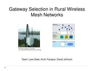
5. Properties of Wireless Mesh Networks • Nodes: • Wireless but static • Connected in an ad-hoc manner • Energy a non-issue (nodes generally plugged in, or easily rechargeable) • Network: • Topology is cluster-based: • Static routers connect subsets of the network. • Routers can serve as source nodes for sub-trees (useful for topology construction, scheduling, etc.)

6. Why Broadcasting in WMNs • Motivation: • Carried over from wired networks • Useful for many applications: • OS updates • Video conferencing/streaming • Multiplayer gaming • Have fewer packet transmissions due to “wireless broadcast advantage” (WBA)

7. What is Wireless Broadcast Advantage (WBA)? • Refers to a unique quality belonging to wireless networks • Wired networks perform broadcast by separate unicasts across the network (separate to each root node in a tree) • In wireless networks: • Direct neighbours of the source node require only one tx • Multiple unicast tx in wired = 1 broadcast tx in wireless Potential Energy and bandwidth savings!

8. Exploiting WBA for Broadcast • Achievement of WBA in broadcast transmissions  configuration changes at link level • Link level changes involve: • Number of radios/channels • Rates • Radio power (for channel reuse) • Antenna gain (direction)

9. Node Configuration • Various node configurations in literature • Authors discuss the following two configurations: • Single-radio single-channel multi-rate • Multi-radio multi-channel multi-rate

10. What is Minimum Latency Broadcasting (MLB)? • Definition: • To provide the best QoS by minimizing latency at the slowest node • Goal: • All destination nodes must receive packet within same time frame • Maximize the transmission rate of the slowest node • Metric: • RAP (Rate-Area Product)

11. Why do we care about MLB? • Motivation: • Want to guarantee quality of service (QoS) to all users in the multicast session • Want to decrease the latency encountered by the slowest link.

12. Overview of Techniques • Both techniques involve the idea of using multicasts across partitioned nodes to achieve broadcast • Single-channel multi-rate: • Also known as “fully multi-rate multicast” (FFM) • Multi-channel multi-rate: • Referred to as the “single best-rate multicast” (SBM)

13. Multi-rate vs. Multi-radio • FMM: • Uses an optimum rate per link to maximize throughput and minimize latency • Attempts to minimize the number of transmissions • Needs scheduling per transmission to avoid interference • SBM: • Determines a single best-rate metric for the entire network • Simplifies the construction algorithm by using one rate • Uses multiple channels, thus simplifying the scheduling algorithm

14. What about Energy Efficiency? • Both techniques transmit a packet multiple times from the same node: • Multi-rate uses multiple rates for various neighbours (based on RAP) • Multi-channel uses multiple channels (channel diversity  non-interference) • The goal: To minimize broadcast latency, not energy efficiency

15. Fully Multi-rate Multicasting (FMM)

16. Fully Multi-rate Multicasting (FMM) • Topic Layout: • What is fully multi-rate multicast? • Why we want to use it • How it works • Topology Construction Algorithm • Multicast Grouping Algorithm • (Simplified) Transmission Scheduling • Maximum end-to-end throughput • Pros and Cons • Recap

17. What is “Fully Multi-Rate Multicast” ? • Broadcast achieved via sequential multicasts • Multicast to separate subsets in network • Algorithm in four steps: • Construct a tree to span the entire network • Calculate the optimum rate at every link • Provide scheduling for all transmissions • Recalculate maximum end-to-end throughput • Caveat: Most of the solutions are NP-hard

18. Why choose FMM • Motivation: • Multi-rate allows us to minimize the MLB • Current radios work with setup • RAP metric is easy to calculate

19. Current 802.11 metrics • Transmit rates and ranges for 802.11b • Obtained via Qualnet simulation • Consider network topology in next slide

20. A Motivational Example • Node 1 wants to broadcast to 2, 3, 4 and 5. • Node 2 @ 11 Mbps, node 5 @ 1 Mbps • One single transmission at lowest rate or two transmissions (one at either rate)

21. Motivational Example: The Single Transmission Case • Node 1 broadcasts to nodes 2 and 5 • Transmission rate = slowest link i.e. 1Mbps • Transmission to node 2 @ 1Mbps  4 is starved until 33 u.t.

22. Motivational Example: The Multiple Transmission Case • Node 1 makes two transmissions • Transmission 1 to node 2 @ 11 Mbps • Transmission sequence: 2  3  4 • Node 1  5 only occurs when 2  3 is complete • Node 4 receives packet at 23 u.t.

23. Topology Construction in FMM • We want to reach all nodes within the network: • Build a connected dominating set (CDS): • Def’n of CDS: • In a graph G(v,e), the connected-dominating set is a set of edges S{e} | all non-leaf nodes v are connected. All other (leaf) nodes are one hop away from at least one node in CDS

24. Connected-Dominating Set (CDS) • What this means: • In a CDS, the source has a path to all relaying nodes in the network • Calculate all possible CDSs in the network • Obtain the CDS with the minimum cost • Steps: • Calculate the set of possible CDSs • Attach a cost metric per CDS • Pick one that minimizes that cost (use Djikstra)

25. Problems with CDS • Problem 1: • For k nodes, 2k possible sets to consider • Solution: • Use Djikstra with an approximation criteria • Problem becomes polynomial • Problem 2: • Minimum connected set will assume slowest rate to maximize downlink neighbours per node • Same as using slowest rate for all nodes • Solution: • Account for the rate metric: max (no. of nodes x transmission rate) • This is defined by the RAP

26. Topology Construction in FMM • Algorithm steps: • Keep a set C of all covered nodes. • C starts with just source node s • Pick optimal product of rate x no. of nodes covered • Add covered nodes within optimal area to C • Continue until C satisfies CDS quality for G • This process ensures a minimum-cost, minimum-spanning tree

27. Sample Network Topology

28. Example: Minimum WCDS Tree

29. Example: Minimum WCDS Tree with rates

30. Multicast Grouping in FMM • Once the broadcast tree is constructed, need to determine two things for each node: • No. of times to multicast • No. of nodes covered by multi-cast • Need to find transmission delay to reach all downstream nodes with minimum latency • Every node’s latency depends on what happens downstream  follow bottom-up topology

31. Bottom-up Topology • Algorithm Steps: • Start with leaf nodes • Calculate the minimum latency to the relay (based on optimal rate in previous step) • Latency maximum at relay node is stored in Cardinality Value (CV) • CV helps determine the transmission delay at relay node R

32. Example: Multicast Grouping

33. Example: Multicast Grouping

34. Example: Multicast Grouping

35. Example: Multicast Grouping

36. Example: Multicast Grouping

37. Bottom-up Topology (2) • CV values along nodes build up a transmission sequence • For k rates, there are 2k-1 possible valid transmission sequences (VTS) • Pick the VTS with the shortest possible transmission delay • Assumption • Grouping does not deal with nodal interference

38. (Simplified) Transmission Scheduling • Transmission sequence determined by CV • Higher CV = higher latency  more critical transmission • All nodes assigned a start-time and a stop time • Nodes must have packet before start time • The goal is to avoid nodal interference • In our example, time is measured in packet time: • Packet tx @ 11 Mbps = 1 u.t.

39. Example: Transmission Scheduling

40. Example: Transmission Scheduling

41. Example: Transmission Scheduling

42. Example: Transmission Scheduling

43. Example: Transmission Scheduling

44. Problems with Transmission Scheduling • Problem 1: • Absolute times require centralized clock • Solution: • Algorithm assumes a centralized clock within source node • Problem 2: • Node schedules are broadcast throughout the network.. to set up broadcasting • Solution 2: • ...........

45. Pros and Cons • Advantages • Obtains lower latency compared to standard techniques • Works with current hardware • Disadvantages: • Algorithms are NP-hard • Scheduling problem has no apparent solution

46. Recap • The technique FMM: • uses selected multicasts to achieve broadcast over network • Minimizes latency in the network • Algorithms required to achieve optimal solution = NP-hard • Need a centralized station for clock synchronization + scheduling • The next technique resolves some of these issues

47. Single Best-Rate Multicasting (SBM)

48. Single Best-rate Multicast (SBM) • Decides a single transmission rate for all link layer data multicast. • Depends on the network's topological properties. • Simplifies broadcasting algorithms.

49. Decisions To Be Made • Selecting 'best' transmission rate to use for all link layer broadcasts. • Deciding whether a certain node should transmit. • Deciding 'Interface Grouping'. • Scheduling each node's transmissions.

50. 'Best' link-layer multicast rate selection • Can be predicted reasonably by the product of the transmission rate and transmission coverage area (rate-area product or RAP). • Higher RAP means more broadcast-efficient for SR-SC MR WMNs.