Download
1 / 32
320 likes | 494 Views
95503 統資軟體課程講義. Functions in Maple. 教授:蔡桂宏 博士 學生:柯建豪 學號 : 95356026. 1.1 Introduction. Understanding functions in Maple is also a good starting point for our discussions about Maple programming.

E N D
95503統資軟體課程講義 Functions in Maple 教授:蔡桂宏 博士 學生:柯建豪 學號:95356026
1.1 Introduction • Understanding functions in Maple is also a good starting point for our discussions about Maple programming. • There are two distinct ways to represent mathematical functions in Maple. That is Maple expression ( := ) and a Maple function ( -> ).
1.2 Functions in Mathematics • the formula has as its domain the set of all real numbers, its codomain is the set of all positive real numbers. • the formula has as its domain the set of all positive real numbers, its codomain is the set of all positive real numbers. • the formula has as its domain the set of all negative real numbers, its codomain is the set of all positive real numbers.
the function f is not invertible. • The inverse of the function g is . • The inverse of the function h is . • So f, g, and h all have the same formula (i.e., rule) but they are not the same function. The domain and codomain are important parts of the definition of a mathematical function.
1.3 Functions in Maple • These two ways of representing mathematical functions are not equivalent. And it is subtle and non-obvious. • A Maple function is something defined using arrow notation ( ->). • A Maple expression is something defined using ( := ). • x -> x^2; • x -> a*x^2; • (x,a) -> a*x^2;
. • Maple will treat all unassigned names (i.e., all unknowns) as variables. • The mathematical function . • g := x -> x^2 – 1;g(2); • g(x) := x^2-1;g(2);
g := cos + ln; • k := x -> cos(x) + ln(x); • g(Pi); k(Pi); • h := cos + (x -> 3*x-1); • h(z);
f := x -> (1 + x^2)/x^3; • g := (1 + (x -> x^2))/(x -> x^3); • h := (1 + (z -> z^2))/(y -> y^3); • f(1); g(1); h(1); • m := x -> (1 + exp(x))/x^3; • n := (1 + exp)/(x -> x^3); • m(1); n(1);
f := x^2; • g := x -> 2 * x^3 * f; • g(x); g(2); • f := x -> x^2; • g := 2 * (x -> x^3) * f; • g(x); g(2);
1.4 Expressions vs. functions: Some puzzles • The following examples are meant to show that there are still a lot of subtle things to learn about variables and functions and how Maple handles them.
Puzzle 1 • f1 := x^2+1; • f2 := y^2+1; • f3 := f1 + f2; • f3 is a function of two variables. • g1 := x -> x^2+1; • g2 := y -> y^2+1; • g3 := g1 + g2;g3(x); • g3 is not a function of two variables.
Puzzle 2 • x:='x': a:=1: b:=2: c:=3: • a*x^2+b*x+c; • f := unapply( a*x^2+b*x+c, x ); • g := x -> a*x^2+b*x+c; • f(x); g(x); • D(f); D(g); • p := x^2 + sin(x) + 1; p(2); • p := unapply(p,x); p(2);
Puzzle 3 • plot( x^2, x=-10..10 ); • plot( x->x^2, -10..10 ); • plot( x^2, -10..10 ); • plot( x->x^2, x=-10..10 );
x := 5; • plot( x^2, x=-10..10 ); • plot( x->x^2, -10..10 );
Puzzle 4 • f := x^2; • f := x*f; • f; • g := x -> x^2; • g := x -> x*g(x); • g(x);
Puzzle 5 • x^2; • f := %; • plot( f, x=-3..3 ); • x^2; • g := x -> %; • plot( g, -3..3 );
1.5 Working with expressions and Maple functions (review) • g := x -> x^2-3*x-10; • g(x); • g; • print(g); • eval(g); • op(g);
plot( a*x^2, -5..5 ); • plot( x->a*x^2, -5..5 ); • plot3d( (x,a)->a*x^2, -5..5, -10..10 );
We wanted to evaluate our mathematical function at a point, say at 1. • f := x^2 - 3*x-10; • g := x -> x^2-3*x-10; • subs( x=1, f ); • eval( f, x=1 ); • g(1); • f(1); • subs( x=1, g );
eval( f, x=1 ); subs( x=1, f ); • Think of reading eval( f, x=1) as " evaluate f at x=1" and think of reading subs (x=1,f) as " substitute x=1 into f". • factor( f ); • factor( g(x) ); • factor( f (x) ); • factor( g );
diff( f, x ); • D( g ); • diff command needed a reference to x in it but the D command did not. • D( f ); • diff( g, x );
Let us do an example of combining two mathematical functions f and g by composing them to make a new function . For the expression: • f := x^2 + 3*x; • g := x + 1; • h := subs( x=g, f ); • subs(x=1, h);
For the function: • f := x -> x^2 + 3*x; • g := x -> x + 1; • h := f@g; • h(x); • h(1);
Let us do an example of representing a mathematical function of two variables. Here is an expression in two variables. • f := (x^2+y^2)/(x+x*y); • g := (x,y) -> (x^2+y^2)/(x+x*y); • subs( x=1, y=2, f ); • eval( f, {x=1, y=2} ); • g(1,2); • simplify( f ); • simplify( g(x,y) );
Here is how we compute partial derivatives of the expression. • diff( f, x ); • simplify( % ); • diff( f, y ); • simplify( % ); • D[1](g); • simplify( %(x,y) ); • D[2](g); • simplify( %(x,y) );
1.6 Anonymous functions and expressions (review) • Here we define an anonymous function and then evaluate, differentiate, and integrate it. • (z -> z^2*tan(z))(Pi/4); • x -> x^3 + 2*x; • %(2); • D( %% ); • int( (%%%)(x), x );
These next two commands show again that defining a function and naming a function are two distinct steps. • z -> z/sqrt(1-z); • f := %;
f := ((x,y) -> x^2) + ((x,y) -> y^3); • f(u,v); • f(2,3); • g := (x -> x^2) + (y -> y^3); • g(u,v); • g(2,3);
plot(w^3+1, w=-1..1); • plot( ((x,y)->x^3-y^3)(w,-1), w = -1..1 ); • plot( w->(((x,y)->x^3-y^3)(w,-1)), -1..1 );
1.7. Functions that return a function (optional) • f := a -> ( y->a*y ); • f(3); • f(3)(4);
f := (x,y) -> 3*x^2+5*y^2; • f(x,3); • fx3 := x -> f(x,3); • fx3(x); • slice_f_with_y_fixed := c -> ( x->f(x,c) ); • fx3 := slice_f_with_y_fixed(3); • fx3(x);