Download
1 / 45
450 likes | 577 Views
The MORPH Algorithm. MORPH = MO dule guided R anking of candidate P at H way genes high throughput data Slides: Rachel E. Bell , June 2013. Motivation. Challenges in studying biological pathways Identify missing pathway members Information gaps on participating genes:

E N D
The MORPH Algorithm MORPH = MOdule guided Ranking of candidate PatHwaygenes high throughput data Slides: Rachel E. Bell, June 2013
Motivation Challenges in studying biological pathways Identify missing pathway members Information gaps on participating genes: e.g. nature of interactions between metabolites and gene expression understanding control mechanisms, feedback, cross-talk Many genes in genome(s) have unknown function
Biological Pathways: Overview What is a pathway? A series of interactions between genes (proteins) involved in performing a certain biological function Cell input = extracellular/ endogenous: e.g.: stress, changes in PH, UV exposure, nutrients Cell output = response: e.g.: transcription of genes, sucrose degradation
MORPH Algorithm: Overview ALGORITHM OUTPUT INPUT High throughput data of gene expression, networks and biological pathways Predict genes involved in biological pathways • Machine learning and validation methods
Other methods for functional prediction Coexpression-based methods (& possibly pathways) e.g.: ACT, GeneCat, ATED-II, MapMan Assumptions: 1) Similar expression patterns -> similar function or regulation 2) Pathway genes -> coordinated expression Network-based methods (& gene expression) e.g: Markov random field (MRF) models , k-nearest neighbours (k-NN), ADOMETA: coexpression, phylogeny, clustering on chrom., metabolic networks Assumption: Closer nodes -> common functions
Introduction: MORPH Algorithm MORPH uses pathway information, gene expression data and network information Compared to other methods, MORPH: • offers robustness (performs well on many pathways) • increases networks coverage • applied to different organisms
Talk outline • MORPH input types: (a) gene expression data, (b) pathways and (c) networks • Types of clustering (modules) methods • The MORPH algorithm and validation • Results • Comparison to other methods • Summary
MORPH Introduction Arabidopsis Thaliana SolanumLycopersicum (Tomato) MORPH was developed on 2 model organisms
MORPH Input: Arabidopsis Thaliana Pathways: 66 AraCyc, 164 MapMan Preprocessing: filter pathways with <10 genes with expression data Total 230 pathways, 2 sets Gene Expression datasets: seedlings, tissues (leaves, roots, flowers, seeds), seed developmental stages, DS1 Preprocessing: filter low variance and detection call, average replicates, normalize to controls, standardize experiments Total 216 GE profiles, 4 datasets, ~12500 genes
MORPH Input: Arabidopsis Thaliana Metabolic (MD) Network (AraCyc) Node = metabolic genes (enzymes) Edges = nodes share a metabolite (reactant or product) Preprocessing: remove most common metabolites (they connect enzymes with weak functional associations) Total: 1987 genes, 56244 interactions PPI Network (PAIR & Interactome Map databases) Node = genes (proteins) Edges = interactions between proteins Preprocessing: Unite (predicted & expt.) interactions from both databases Total: 4642 genes, 149229 interactions
Talk outline MORPH input types: (a) gene expression data, (b) pathways and (c) networks Types of clustering (modules) methods The MORPH algorithm and validation Results Comparison to other methods Summary
MORPH Goal MORPH goal: Given a specific biological pathway MORPH seeks candidate genes that participate in (or regulate) the pathway. MORPH receives 3 types of input: Pathways Gene expression data Partitioning into modules A key step in MORPH is the partitioning of genes into modules (clusters).
Assumptions of clustering data into modules Q: Why use modules? Modules reflect broad functions Some functions are related to target pathway Pathway genes -> more coordinated expression than random genes
Input: Partitioning Gene Modules and Networks Different strategies for partitioning genes Expression based clustering Network based clustering Annotation based clustering • Enzyme/not enzyme Orthologsin rice & maize/no orthologs Matisse* SOM = self-organizing map (partitions all genes) CLICK = CLusterIdentification via Connectivity Kernels (partitions most genes) Markov cluster algorithm (MCL)
Interaction High expression similarity Input: Partitioning Networks Reminder: MATISSE seeks connected sub-networks with high expression similarity (Ulitsky & Shamir, 2007) Goal: construct modules using gene expression data and networks Problem: low coverage of MD network
Input: Partitioning Networks - MATISSE* Motivation - overcome low coverage of networks • Add genes with high correlation • Repeat until module correlation <0.4 • Connectivity ignored MATISSE* (modified MATISSE) Results: Matisse* increased MD network coverage to ~4500 genes Matisse* performed similarly to Matisse
Summary: Methods of Partitioning Gene Modules and Networks Annotation-based clustering Gene expression-based clustering Modules using network data Total of 8 clustering solutions
Talk outline MORPH input types: (a) gene expression data, (b) pathways and (c) networks Types of clustering (modules) methods The MORPH algorithm and validation Results Comparison to other methods Summary
MORPH = MOdule guided Ranking of candidate PatHway genes MORPH is an algorithm for prioritizing novel candidate genes in a given specific pathway. Input: • Pathway genes S = {s1,s2,…sl} • Gene expression profiles • Partition solution for genes with gene expression data: k modules = M1……Mk • Similarity function (D) Pearson/Spearman
Module-Guided Ranking Algorithm Step #1: Partition genes into k modules M1,M2,…,Mk #2 #3 #1 • Step #2: • Identify pathway genes s1,s2,…,sland candidate genes g • ignore modules with no pathway genes • add module for non partitioned pathway genes Step #3: Analyze each module separately
Module-Guided Ranking Algorithm #4 #3 Step #4: For each g(candidate gene) in module Mi calculate mean similarity with sj (pathway genes) using gene expression data candidate genes pre-defined module Similarity function (Pearson’s Corr.) pathway genes in module provides ranking within module
Module-Guided Ranking Algorithm Step #5: Standardize mean similarity scores within each module mean similarity scores of all candidate genes in module Mi candidategenes stdev / mean of #6 Step #6: Rank all candidate genes (using standardized z-scores) #5
How do we assess predictions of many pathways? Given a clustering solution AND gene dataset run algorithm for each pathway Arabidopsis Thaliana230 pathways Assessment of pathways using Leave-One-Out Cross-Validation (LOOCV) procedure
Leave-One-Out Cross-Validation (LOOCV) procedure LOOCV generates for each pathway gene -> SELF-RANK Definition SELF RANK of a gene is its position in ranking, when left out of algorithm calculation Meaning Self rank of pathway gene = its overall strength of association with remaining pathway genes Kharchenko et al., 2006
Self-Rank Curve: AUSR score LOOCV procedure For each pathway S: Remove one gene (v) -> S\{v} Consider S\{v} = test set Generate ranking of v using S\{v} Repeat for every v (Random gene set of size 13 genes) AUSR score assesses pathway solutions (given input combinations – discussed next) • Calculate self-rank for all v in S • Create self-rank plot • Self-rank threshold of k=1..1000 • Calculate area under self-rank curve (AUSR) (k) Figure 2 Self-Rank plot of the Carotenoid Biosynthetic Pathway contains 13 genes; SOM - clustering solution
Talk outline MORPH input types: (a) gene expression data, (b) pathways and (c) networks Types of clustering (modules) methods The MORPH algorithm and validation Results Comparison to other methods Summary
Different input produces different AUSR scores FIGURE 3: Comparison of 2 gene expr. datasets AUSR(seedlings) - AUSR(DS1) Different: gene expression dataset Same: MD network, Matisse*, 66 AraCyc Pathways Inspired adoption of selection (learning configuration)
Learning Configuration Every pathway tested with gene expression dataset and partitioning solution (modules) Definition Learning configuration = combination of: gene expression dataset (4) AND Clustering solution (8) Total of 4x8 = 32 combinations
Machine Learning MORPH applies a selection procedure LOOCV used to select optimal learning configuration (i.e. data set and clustering) for each examined pathway. LOOCV avoids overfitting, since test gene is left out.
Comparison of selection process to other ‘fixed’ configurations 66 AraCyc metabolic pathways • Results • Better: enzymes or MD network • Poorer: PPI network, no clustering, SOM, CLICK & Orthologs • (metabolic genes had higher corr.) • Selection improved on all configurations Figure 4: The average AUSR for each learning combination (gene expr. dataset + clustering solution)
Robustness of selection method 66 AraCyc pathways 1.5 Real vs. Random Pathways randomly selected sets with same size (repeated 100 times for each size) Results 29/66 AUSR > maximal random score AUSR > 0.75 15/66 - real pathways 0 - random 1.0 AUSR 0.5 0.0 Sizes Figure 5: AUSR Scores of Real and Random Pathways
Talk outline MORPH input types: (a) gene expression data, (b) pathways and (c) networks Types of clustering (modules) methods The MORPH algorithm and validation Results Comparison to other methods Summary
Comparison of MORPH to other methods: Arabidopsis Thaliana pathways 66 AraCyc Pathways * Coexpression (no network data) methods using reference datasets: ACT, DS1 Markov Ranking Field (MRF) methods (network data) CMRF = total # of pathway gene in neighbourhood WMRF= total similarity with path. genes in neighbourhood 164 MapManPathways * k-Nearest Neighbour (k-NN) (network data) Input: Gene expression: seeds, tissues, seedlings, DS1 Networks: PPI and MD networks Pathways: AraCyc, MapMan Figures 4B & 4C
Figure 4D & 4E: Comparison to other methods AraCycpathways with AUSR>0.8 MapMan pathways with AUSR>0.7 k-NN predictor complements MORPH
My analysis: AUSR scores of MORPH and k-NN Data retrieved from Supplemental Data Set 3 k-NN is twice as good as MORPH for high AUSRs >0.9 (6 compared to 3)
Carotenoid Pathway and the MORPH Candidate genes • Carotenoids are antioxidants, perform stress response functions • Candidate Genes (Numbered Octagons) • 8/25 top candidates have predicted functions, with little details of roles in plants • Other predictions inc. genes with similar functions – response to oxidative stress SPS2 – Plastoquinone pathway essential for carotenoid pathway SQE3 –catalyzes the precursor of a pathway which is coordinated expression with the carotenoid pathway
Comparison of MORPH to other methods 93 Tomato pathways Figure 7 Predictors include MORPH, k-NN, MRF-based, and coexpression based classifiers. (A) Average and median AUSR scores. (B) The number of pathways that had AUSR score above 0.7
Talk outline MORPH input types: (a) gene expression data, (b) pathways and (c) networks Types of clustering (modules) methods The MORPH algorithm and validation Results Comparison to other methods Summary
Summary: Advantages of MORPH • Robust – different pathways • k-NN consider only genes in the network, MORPH increases network coverage • k-NN more dependent on sub-networks diameter (higher diameter lower AUSR), MORPH more robust • Self-rank k=1000 threshold for AUSR, ignores poor pathway gene correlations • Potential useful predictions
Summary: Drawbacks of MORPH • If pathway genes not coherent, better select best/top module(s) than average • Dependent on input quality (e.g. AraCyc > MapMan) • Predicts close pathways (drawback/advantage) • Requires known pathway info for predictions
MORPH Classifications 3 types of input data: Pathways genes (s1,s2,…sl) Gene expression Partition gene expression data into k modules = M1,…,Mk 66 Arabidopsis Thaliana 4 datasets 8 Partitioning methods