Download

1 / 58
580 likes | 747 Views
Analyzing Non-Normal Data with Generalized Linear Models 2010 LISA Short Course Series. Sai Wang, Dept. of Statistics. Presentation Outline. 1. Introduction to Generalized Linear Models 2. Binary Response Data - Logistic Regression Model Ex. Teaching Method

E N D
Analyzing Non-Normal Data with Generalized Linear Models2010 LISA Short Course Series Sai Wang, Dept. of Statistics
Presentation Outline 1. Introduction to Generalized Linear Models 2. Binary Response Data - Logistic Regression Model Ex. Teaching Method 3. Count Response Data - Poisson Regression Model Ex. Mining Example 4. Non-parametric Tests
Normal: continuous, symmetric, mean μ and varσ2 Bernoulli: 0 or 1, mean p and var p(1-p) special case of Binomial Poisson: non-negative integer, 0, 1, 2, …, mean λvarλ # of events in a fixed time interval
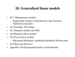
Generalized linear models (GLM) extend ordinary regression to non-normal response distributions. Response distribution must come from the Exponential Family of Distributions Includes Normal, Bernoulli, Binomial, Poisson, Gamma, etc. 3 Components Random – Identifies response Y and its probability distribution Systematic – Explanatory variables in a linear predictor function (Xβ) Link function – Invertible function (g(.)) that links the mean of the response (E[Yi]=μi) to the systematic component. Generalized Linear Models
Model for i =1 to n, where n is # of obs j= 1 to k, where k is # of predictors Equivalently, Generalized Linear Models
Why do we use GLM’s? Linear regression assumes that the response is distributed normally GLM’s allow us to analyze the linear relationship between predictor variables and the mean of the response variable when it is not reasonable to assume the data is distributed normally. Generalized Linear Models
Connection Between GLM’s and Multiple Linear Regression Multiple linear regression is a special case of the GLM Response is normally distributed with variance σ2 Identity link function μi= g(μi) = xiTβ Generalized Linear Models
Predictor Variables Two Types: Continuous and Categorical Continuous Predictor Variables Examples – Time, Grade Point Average, Test Score, etc. Coded with one parameter – βjxj Categorical Predictor Variables Examples – Sex, Political Affiliation, Marital Status, etc. Actual value assigned to Category not important Ex) Sex - Male/Female, M/F, 1/2, 0/1, etc. Coded Differently than continuous variables Generalized Linear Models
Predictor Variables cont. Consider a categorical predictor variable with L categories One category selected as reference category Assignment of reference category is arbitrary Some suggest assign category with most observations Variable represented by L-1 dummy variables Model Identifiability Generalized Linear Models
Predictor Variables cont. Two types of coding Dummy Coding (Used in R) xk = 1 If predictor variable is equal to category k 0 Otherwise xk = 0 For all k if reference category Effect Coding (Used in JMP) xk = 1 If predictor variable is equal to category k 0 Otherwise xk = -1 For all k if predictor variable is reference category Generalized Linear Models
Model Evaluation - -2 Log Likelihood Specified by the random component of the GLM model For independent observations, the likelihood is the product of the probability distribution functions of the observations. -2 Log likelihood is -2 times the log of the likelihood function -2 Log likelihood is used due to its distributional properties – Chi-square Generalized Linear Models
Saturated Model (Perfect Fit Model) Contains a separate indicator parameter for each observation Perfect fit μi = yi Not useful since there is no data reduction i.e. number of parameters equals number of observations Maximum achievable log likelihood (minimum -2 Log L) – baseline for comparison to other model fits Generalized Linear Models
Deviance Let L(β|y) = Maximum of the log likelihood for a proposed model L(y|y) = Maximum of the log likelihood for the saturated model Deviance = D(β) = -2 [L(β|y) - L(y|y)] Generalized Linear Models
Deviance cont. Generalized Linear Models Model Chi-Square
Deviance cont. Lack of Fit test Likelihood Ratio Statistic for testing the null hypothes is that the model is a good alternative to the saturated model Has an asymptotic chi-squared distribution with N – p degrees of freedom, where p is the number of parameters in the model. Also allows for the comparison of one model to another using the likelihood ratio test. Generalized Linear Models
Nested Models Model 1 - Model with p predictor variables {X1, X2…,Xp} and vector of fitted values μ1 Model 2 - Model with q<p predictor variables {X1, X2,…,Xq} and vector of fitted values μ2 Model 2 is nested within Model 1 if all predictor variables found in Model 2 are included in Model 1. i.e. the set of predictor variables in Model 2 are a subset of the set of predictor variables in Model 1 Generalized Linear Models
Nested Models Model 2 is a special case of Model 1 - all the coefficients corresponding to Xq+1, Xq+2, Xq+3,….,Xpare equal to zero Generalized Linear Models
Likelihood Ratio Test Null Hypothesis for Nested Models: The predictor variables in Model 1 that are not found in Model 2 are not significant to the model fit. Alternate Hypothesis for Nested Models - The predictor variables in Model 1 that are not found in Model 2 are significant to the model fit. Generalized Linear Models
Likelihood Ratio Test Likelihood Ratio Statistic = -2L(y, μ2) - (-2L(y, μ1)) = D(y,μ2) - D(y, μ1) Difference of the deviances of the two models Always D(y,μ2) > D(y,μ1) implies LRT > 0 LRT is distributed Chi-Squared with p-q degrees of freedom Later, the Likelihood Ratio Test will be used to test the significance of variables in Logistic and Poisson regression models. Generalized Linear Models
Theoretical Example of Likelihood Ratio Test 3 predictor variables – 1 Continuous (X1: GPA), 1 Categorical with 4 Categories (X2, X3, X4, Year in college), 1 Categorical with 2 Category (X5: Sex) Model 1 - predictor variables {X1, X2, X3, X4, X5} Model 2 - predictor variables {X1, X5} Null Hypothesis – Variables with 4 categories is not significant to the model (β2 = β3 = β4= 0) Alternate Hypothesis - Variable with 4 categories is significant Generalized Linear Models
Theoretical Example of Likelihood Ratio Test Cont. Likelihood Ratio Test Statistic = D(y,μ2) - D(y, μ1) Difference of the deviance statistics from the two models Equivalently, the difference of the -2 Log L from the two models Chi-Squared Distribution with 5-2=3 degrees of freedom Generalized Linear Models
Model Comparison Determining Model Fit cont. Akaike Information Criterion (AIC) Penalizes model for having many parameters AIC = -2 Log L +2*p where p is the number of parameters in model, small is better Bayesian Information Criterion (BIC) BIC = -2 Log L + ln(n)*p where p is the number of parameters in model and n is the number of observations Usually stronger penalization for additional parameter than AIC Generalized Linear Models
Summary Setup of the Generalized Linear Model Continuous and Categorical Predictor Variables Log Likelihood Deviance and Likelihood Ratio Test Test lack of fit of the model Test the significance of a predictor variable or set of predictor variables in the model. Model Comparison Generalized Linear Models
Questions/Comments Generalized Linear Models
Consider a binary response variable. Variable with two outcomes One outcome represented by a 1 and the other represented by a 0 Examples: Does the person have a disease? Yes or No Outcome of a baseball game? Win or loss Logistic Regression
Teaching Method Data Set Found in Aldrich and Nelson (Sage Publications, 1984) Researcher would like to examine the effect of a new teaching method – Personalized System of Instruction (PSI) Response variable is whether the student received an A in a statistics class (1 = yes, 0 = no) Other data collected: GPA of the student Score on test entering knowledge of statistics (TUCE) Logistic Regression
Consider the linear probability model where yi = response for observation i xi = 1 x p vector of covariates for observation i p = 1+k, number of parameters Logistic Regression
GLM with binomial random component and identity link g(μ) = μ Issues: pi can take on values less than 0 or greater than 1 Predicted probability for some subjects fall outside of the [0,1] range. Logistic Regression
Consider the logistic regression model GLM with binomial random component and logit link g(μ) = logit(μ) Range of values for pi is 0 to 1 Logistic Regression
Interpretation of Coefficient β – Odds Ratio Odds: fraction of Prob(event)=p vsProb(not event)=1-p The odds ratio is a statistic that measures the odds of an event compared to the odds of another event. Ex. Say the probability of Event 1 is p1and the probability of Event 2 is p2. Then the odds ratio of Event 2 to Event 1 is: Logistic Regression
Interpretation of Coefficient β – Odds Ratio Cont. Logistic Regression
Interpretation of Coefficient β – Odds Ratio Cont. Value of Odds Ratio range from 0 to Infinity Value between 0 and 1 indicate the odds of Event 1 are greater Value between 1 and infinity indicate odds of Event 2 are greater Value equal to 1 indicates events are equally likely Logistic Regression
Interpretation of Coefficient β – Odds Ratio Cont. Link to Logistic Regression : Thus the odds ratio of event 2 to event 1 is Note: One should take caution when interpreting parameter estimates Multicollinearity can change the sign, size, and significance of parameters Logistic Regression
Interpretation of Coefficient β – Odds Ratio Cont. Consider Event 1 is Y=1 given X (prob=p1) and Event 2 is Y=1 given X+1 (prob=p2) From our logistic regression model Thus the odds ratio of Y=1 for per unit increase in X is Logistic Regression
Interpretation for a Continuous Predictor Variable Consider the following JMP output: Parameter Estimates Term Estimate Std Error L-R ChiSquareProb>ChiSq Lower CL Upper CL Intercept -11.832 4.7161554 9.9102818 0.0016* -23.38402 -3.975928 GPA 2.8261126 1.2629411 6.7842138 0.0092* 0.6391582 5.7567314 TUCE 0.0951577 0.1415542 0.4738788 0.4912 -0.170202 0.4050175 PSI[0] -1.189344 0.5322821 6.2036976 0.0127* -2.40494 -0.239233 Interpretation of the Parameter Estimate: exp2.8261125 = 16.8797 = Odds ratio between the odds at x+1 and odds at x for any gpa score The ratio of the odds of getting an A between a person with a 3.0 gpa and 2.0 gpa is equal to 16.8797 or in other words the odds of the person with the 3.0 is 16.8797 times the odds of the person with the 2.0. Equivalently, the odds of NOT getting an A for a person with a 3.0 gpa is equal to 1/16.8797 =0.0592 times the odds of NOT getting an A for a person with a 2.0 gpa. Logistic Regression
Single Categorical Predictor Variable Consider the following JMP output: Parameter Estimates Term Estimate Std Error L-R ChiSquareProb>ChiSq Lower CL Upper CL Intercept -11.832 4.7161554 9.9102818 0.0016* -23.38402 -3.975928 GPA 2.8261126 1.2629411 6.7842138 0.0092* 0.6391582 5.7567314 TUCE 0.0951577 0.1415542 0.4738788 0.4912 -0.170202 0.4050175 PSI[0] -1.189344 0.5322821 6.2036976 0.0127* -2.40494 -0.239233 Interpretation of the Parameter Estimate: exp 2*-1.1893 = 0.0928 = Odds ratio between the odds of getting an A for a student that was not subject to the teaching method and for a student that was subject to the teaching method. The odds of NOT getting an A without the teaching method is 1/0.0928=10.7898 times the odds of NOT getting an A with the teaching method. I Logistic Regression
ROC Curve Receiver Operating Curve Sensitivity – Proportion of positive cases (Y=1) that were classified as a positive case by the model Specificity - Proportion of negative cases (Y=0) that were classified as a negative case by the model Logistic Regression
ROC Curve Cont. Cutoff Value - Selected probability where all cases in which predicted probabilities are above the cutoff are classified as positive (Y=1) and all cases in which the predicted probabilities are below the cutoff are classified as negative (Y=0) 0.5 cutoff is commonly used ROC Curve – Plot of the sensitivity versus one minus the specificity for various cutoff values False positives (1-specificity) on the x-axis and True positives (sensitivity) on the y-axis Logistic Regression
ROC Curve Cont. Measure the area under the ROC curve Poor fit – area under the ROC curve approximately equal to 0.5 Good fit – area under the ROC curve approximately equal to 1.0 Logistic Regression
Summary Introduction to the Logistic Regression Model Interpretation of the Parameter Estimates β – Odds Ratio ROC Curves Teaching Method Example Logistic Regression
Questions/Comments Logistic Regression
Consider a count response variable. Response variable is the number of occurrences in a given time frame. Outcomes equal to 0, 1, 2, …. Examples: Number of penalties during a football game. Number of customers shop at a store on a given day. Number of car accidents at an intersection. Poisson Regression
Mining Data Set Found in Myers (1990) Response of interest is the number of fractures that occur in upper seam mines in the coal fields of the Appalachian region of western Virginia Want to determine if fractures is a function of the material in the land and mining area Four possible predictors Inner burden thickness Percent extraction of the lower previously mined seam Lower seam height Years the mine has been open Poisson Regression
Mining Data Set Cont. Coal Mine Seam Poisson Regression
Mining Data Set Cont. Coal Mine Upper and Lower Seams Prevalence of overburden fracturing may lead to collapse Poisson Regression
Consider the model where Yi = Response for observation i xi = 1x(k+1) vector of covariates for observation i p = Number of covariates μi = Expected number of events given xi GLM with Normal random component and identity link g(μ) = μ Issue: Predicted values range from -∞ to +∞ Poisson Regression
Consider the Poisson log-linear model GLM with Poisson random component and log link g(μ) = log(μ) Predicted response values fall between 0 and +∞ In the case of a single predictor, An increase by one unit in x results an multiple of in μ Poisson Regression
Continuous Predictor Variable Consider the JMP output Term Estimate Std Error L-R ChiSquareProb>ChiSq Lower CL Upper CL Intercept -3.59309 1.0256877 14.113702 0.0002* -5.69524 -1.660388 Thickness -0.001407 0.0008358 3.166542 0.0752 -0.003162 0.0001349 Pct_Extraction 0.0623458 0.0122863 31.951118 <.0001* 0.0392379 0.0875323 Height -0.00208 0.0050662 0.174671 0.6760 -0.012874 0.0070806 Age -0.030813 0.0162649 3.8944386 0.0484* -0.064181 -0.000202 Interpretation of the parameter estimate: exp-0.0308 = .9697 = multiplicative effect on the expected number of fractures for an increase of 1 in the years the mine has been opened Poisson Regression
Overdispersion for Poisson Regression Models More variability in the response than the model allows For Yi~Poisson(λi), E [Yi] = Var [Yi] = λi The variance of the response is much larger than the mean. Consequences: Parameter estimates are still consistent Standard errors are inconsistent Detection: D(β)/n-p Large if overdispersion is present Poisson Regression