Download

1 / 40
440 likes | 697 Views
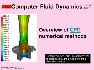
Computer Fluid Dynamics E181107. 2181106. CFD7r. Solvers, schemes SIMPLEx, upwind REDUCED lecture…. Rudolf Žitný, Ústav procesní a zpracovatelské techniky ČVUT FS 2010. z. y. T op. N orth. E. W est. S outh. x. z. y. x. B ottom. x. FINITE VOLUME METHOD. CFD7r.

E N D
ComputerFluid DynamicsE181107 2181106 CFD7r Solvers, schemes SIMPLEx, upwindREDUCED lecture… Rudolf Žitný, Ústav procesní a zpracovatelské techniky ČVUT FS 2010
z y Top North E West South x z y x Bottom x FINITE VOLUME METHOD CFD7r FINITE CONTROL VOLUMEx = Fluid element dx Finite size Infinitely small size
FVM diffusion problem 2D CFD7r N W P eE A S Boundary conditions Example: insulation q=0 • First kind (Dirichlet BC) • Second kind (Neumann BC) • Third kind (Newton’s BC) Example: Finite thermal resistance (heat transfer coefficient )
w e A W P E B FVM convection diffusion 1D CFD7r CV - control volume A – surface of CV Gauss theorem 1D case F-mass flux D-diffusion conductance
FVM convection diffusion 1D CFD7r Relative importance of convective transport is characterised by Peclet number of cell (of control volume, because Pe depends upon size of cell) Thermal conductivity Prandtl Binary diffusion coef Schmidt
FVM convection diffusion 1D CFD7r • Methods differ in the way how the unknown transported values at the control volume faces (w , e) are calculated (different interpolation techniques) • Result can be always expressed in the form • Properties of resulting schemes should be evaluated • Conservativeness • Boundedness (positivity of coefficients anb) • Transportivity (schemes should depend upon the Peclet number of cell)
FVM central scheme 1D CFD7r • Conservativeness (yes) • Boundedness (positivity of coefficients) • Transportivness (no) Very fine mesh is necessary
FVM upwind 1st order 1D CFD7r • Conservativeness (yes) • Boundedness (positivity of coefficients) YES for any Pe • Transportivness (YES) But at a prize of decreased order of accuracy (only 1st order!!)
FVM Upwind FLUENT CFD7r Upwind of the first order Upwind of the second order 1 f 0
FVM exponential FLUENT CFD7r Called power law model in Fluent • Exact solution of Projection of velocity to the direction r 1 r 0 • For Pe<<1 the exponential profile is reduced to linear profile
FVM dispersion / diffusion CFD7r There are two basic errors caused by approximation of convective terms • False diffusion(or numerical diffusion) – artificial smearing of jumps, discontinuities. Neglected terms in the Taylor series expansion of first derivatives (convective terms) represent in fact the terms with second derivatives (diffusion terms). So when using low order formula for convection terms (for example upwind of the first order), their inaccuracy is manifested by the artificial increase of diffusive terms (e.g. by increase of viscosity). The false diffusion effect is important first of all in the case when the flow direction is not aligned with mesh, see example • Dispersion(or aliasing) – causing overshoots, artificial oscillations. Dispersion means that different components of Fourier expansion (of numerical solution) move with different velocities, for example shorter wavelengths move slower than the velocity of flow. Numerical dispersion Numerical diffusion 1 u=v 0 - boundary condition, all values are zero in the right triangle (without diffusion)
FVM Navier Stokes equations CFD7r Different methods are used for numerical solution of Navier Stokes equations at Compressible flows (finite speed of sound, existence of velocity discontinuities at shocks) Incompressible flows (infinite speed of sound) Explicit methods (e.g. MacCormax) but also implicit methods (Beam-Warming scheme) are used. These methods will not be discussed here. Vorticity and stream function methods (pressure is eliminated from NS equations). These methods are suitable especially for 2D flows. Primitive variable approach (formulation in terms of velocities and pressure). Pressure represents a continuity equation constraint. Only these methods (pressure corrections methods SIMPLE, SIMPLER, SIMPLEC and PISO) using staggered and collocated grid will be discussed in this lecture. Beckman
FVM Navier Stokes equations CFD7r Example: Steady state and 2D (velocities u,v and pressure p are unknown functions) This is equation for u This is equation for v This is equation for p? But pressure p is not in the continuity equation!Solution of this problem is in SIMPLE methods, described later
0 0 10 0 10 10 10 10 10 10 10 0 10 0 0 0 0 0 0 0 10 FVM checkerboard pattern CFD7r Other problem is called checkerboard pattern This nonuniform distribution of pressure has no effect upon NS equations The problem appears as soon as the u,v,p values are concentrated in the same control volume W P E
0 0 10 0 10 10 10 10 10 10 10 0 10 0 0 0 0 0 0 0 10 FVM staggered grid CFD7r Different control volumes for different equations Control volume for momentum balance in y-direction Control volume for continuity equation, temperature, concentrations Control volume for momentum balance in x-direction
FVM staggered grid CFD7r Location of velocities and pressure in staggered grid Control volume for momentum balance in y-direction j+2 j+1 j j-1 Control volume for continuity equation, temperature, concentrations J+1 J J-1 J-2 Pressure I,J U i,J V I,j u p v Control volume for momentum balance in x-direction I-2 I-1 I I+1 I+2 i-1 i i+1 i+2
FVM momentum x CFD7r j+2 j+1 j j-1 J+1 J J-1 J-2 Pressure I,J U i,J V I,j u p p Control volume for momentum balance in x-direction I-2 I-1 I I+1 I+2 i-1 i i+1 i+2
FVM SIMPLE step 1 (velocities) CFD7r Input: Approximation of pressure p*
FVM SIMPLE step 2 (pressure correction) CFD7r “true” solution Neglect!!! subtract Substitute u*+u’ and v*+v’ into continuity equation Solve equations for pressure corrections
FVM SIMPLE step 3 (update p,u,v) CFD7r Only these new pressures are necessary for next iteration Continue with the improved pressures to the step 1
FVM SIMPLER (SIMPLE Revised) CFD7r Idea: calculate pressure distribution directly from the Poisson’s equation
FVM Rhie Chow (Fluent) CFD7r The way how to avoid staggering (difficult implementation in unstructured meshes) was suggested in the paper Rhie C.M., Chow W.L.: Numerical study of the turbulent flow past an airfoil with trailing edge separation. AIAA Journal, Vol.21, No.11, 1983 This technique is calledRhie-Chow interpolation.
E P e FVM Rhie Chow (Fluent) CFD7r Rhie C.M., Chow W.L.: Numerical study of the turbulent flow past an airfoil with trailing edge separation. AIAA Journal, Vol.21, No.11, 1983 How to interpolate ue velocity at a control volume face
Fluent - solvers CFD7r Segregated solver Coupled solver , , cp,… , , cp,… u… v… w… p… (SIMPLE…) CFL Courant Friedrichs Lewy criterion k,,…… T,k,,…… Nonstationary problem always solved by implicit Euler Nonstationary problem solved by implicit Euler (CFL~5), explicit Euler (CFL~1) or Runge Kutta Algebraic eq. by multigrid AMG, or FAS (Full Aproximation Storage) Algebraic eq. by multigrid AMG
FVM solvers CFD7r Dalí
FVM solvers CFD7r Solution of linear algebraic equation system Ax=b • TDMA – Gauss elimination tridiagonal matrix (obvious choice for 1D problems, but suitable for 2D and 3D problems too, iteratively along the x,y,z grid lines – method of alternating directions ADI) • PDMA – pentadiagonal matrix(suitable for QUICK), Fortran version • CGM – Conjugated Gradient Method(iterative method: each iteration calculates increment of vector in the direction of gradient of minimised function – square of residual vector) • Multigrid method (Fluent)
Solver TDMA tridiagonal system MATLAB CFD7r function x = TDMAsolver(a,b,c,d) %a, b, c, and d are the column vectors for the compressed tridiagonal matrix n = length(b); % n is the number of rows % Modify the first-row coefficients c(1) = c(1) / b(1); % Division by zero risk. d(1) = d(1) / b(1); % Division by zero would imply a singular matrix. for i = 2:n id = 1 / (b(i) - c(i-1) * a(i)); % Division by zero risk. c(i) = c(i)* id; % Last value calculated is redundant. d(i) = (d(i) - d(i-1) * a(i)) * id; end % Now back substitute. x(n) = d(n); for i = n-1:-1:1 x(i) = d(i) - c(i) * x(i + 1); end end Forward step (elimination entries bellow diagonal)
Solver TDMA applied to 2D problems (ADI) CFD7r Y-implicit step (repeated application of TDMA for 10 equations, proceeds from left to right) X-implicit step (proceeds bottom up) y x
Solver MULTIGRID CFD7r Solution on a rough grid takes into account very quickly long waves (distant boundaries etc), that is refined on a finer grid. Rough grid (small wave numbers) Fine grid (large wave numbers details) Interpolation from rough to fine grid Averaging from fine to rough grid
n+1 n+1 n+1 ∆t ∆t ∆t n n n ∆x ∆x ∆x n-1 n-1 n-1 Unsteady flows CFD7r Discretisation like in the finite difference methods discussed previously Example: Temperature field EXPLICIT scheme IMPLICIT scheme CRANK NICHOLSON scheme First order accuracy in time First order accuracy in time Second order accuracy in time Stable only if Unconditionally stable and bounded Unconditionally stable, but bounded only if
PRESSURE PRESSURE OUTLET PRESSURE INLET INLET PRESSURE PRESSURE OUTLET OUTLET PRESSURE PRESSURE FVM Boundary conditions CFD7r • Boundary conditions are specified at faces of cells (not at grid points) • INLET specified u,v,w,T,k, (but not pressure!) • OUTLET nothing is specified (p is calculated from continuity eq.) • PRESSURE only pressure is specified (not velocities) • WALL zero velocities, kP, P calculated from the law of wall P yP Recommended combinations for several outlets Forbiddencombinations for several outlets there is no unique solution because no flowrate is specified
Stream function-vorticity CFD7r Introducing stream function and vorticity instead of primitive variables (velocities and pressure) eliminates the problem with the checkerboard pattern. Continuity equation is exactly satisfied. However the technique is used mostly for 2D problems (it is sufficient to solve only 2 equations), because in 3D problems 3 components of vorticity and 3 components of vector potential must be solved (comparing with only 4 equations when using primitive variable formulation of NS equations). Ghirlandaio
Stream function-vorticity CFD7r The best method for solution of 2D problems of incompressible flows Pressure elimination Introduction vorticity (z-component of vorticity vector) Velocities expressed in terms of scalar stream function Vorticity expressed in terms of stream function
Stream function-vorticity CFD7r Three equations for u,v,p are replaced by two equations for , . Advantage: continuity equation is exactly satisfied. Vorticity transport is parabolic equation, Poisson equaion for stream function is eliptic. Lines of constant are streamlines (at wall =const). The no-slip condition at wall (prescribed velocities) must be reflected by boundary condition for vorticity How to do it, is shown in the next slide on example of flow in a channel
Stream function-vorticity CFD7r Stream function Increases from 0 to w for example =uy N-1=N M y H N-1 N 2 1 2 x 1 =0 Vorticity Zero vorticity at axis (follows from definition) Prescribed velocity profile at inlet u1(y) and v1(y)=0 Vorticity at wall (prescribed velocity U, in this case zero)
UM M y H N-1 N 2 1 2 x 1 Example: cavity flow 1/4 CFD7r Cavity flow. Lid of cavity is moving with a constant velocity U. There is no in-out flow, therefore stream function (proportional to flowrate) is zero at boundary, at all walls of cavity Vorticity at moving lid Vorticity at fixed walls
UM y N W P E S x Example: cavity flow 2/4 CFD7r FVM applied to vorticity transport equation (upwind of the first order). Equidistant grid is assumed =x=y Eliptic equation for stream function This systém of algebraic equation (including boundary conditions) is to be solved iteratively (for example by alternating direction method ADI described previously)
Example: cavity flow 3/4 CFD7r Matlab % tok v dutině. metoda vířivosti a pokutové funkice. Upwind. Metoda % střídavých směrů. h=0.01; um=0.0001; visc=1e-6; % parametry site, a casovy krok relax=0.5; n=21; d=h/(n-1); d2=d^2; niter=50; psi=zeros(n,n); omega=zeros(n,n); u=zeros(n,n); v=zeros(n,n); a=zeros(n,1); b=ones(n,1); c=zeros(n,1); r=zeros(n,1); for iter=1:niter for i=1:n u(i,n)=um; end for i=2:n-1 for j=2:n-1 u(i,j)=(psi(i,j+1)-psi(i,j-1))/(2*d); v(i,j)=(psi(i-1,j)-psi(i+1,j))/(2*d); end end %stream function x-implicit for j=2:n-1 for i=2:n-1 a(i)=-1/d2;b(i)=4/d2;c(i)=-1/d2; r(i)=(psi(i,j-1)+psi(i,j+1))/d2+ omega(i,j); end r(1)=0;r(n)=0; ps=tridag(a,b,c,r,n); for i=2:n-1 psi(i,j)=(1-relax)*psi(i,j)+relax*ps(i); end end %stream function y-implicit for i=2:n-1 for j=2:n-1 a(j)=-1/d2;b(j)=4/d2;c(j)=-1/d2;r(j)=(psi(i-1,j)+psi(i+1,j))/d2+ omega(i,j); end r(1)=0;r(n)=0; ps=tridag(a,b,c,r,n); for j=2:n-1 psi(i,j)=(1-relax)*psi(i,j)+relax*ps(j); end end % vorticity boundary conditions for i=1:n omega(i,n)=relax*omega(i,n)+(1-relax)*2/d2* (psi(i,n)-psi(i,n-1)-um*d); omega(i,1)=relax*omega(i,1)+(1-relax)*2* (psi(i,1)-psi(i,2))/d2; omega(1,i)=relax*omega(1,i)+(1-relax)*2*(psi(1,i)-psi(2,i))/d2; omega(n,i)=relax*omega(n,i)+(1-relax)*2*(psi(n,i)-psi(n-1,i))/d2; end %vorticity x-implicit for j=2:n-1 for i=2:n-1 up=u(i,j);vp=v(i,j); a(i)=-visc/d2-max(up,0)/d; b(i)=4*visc/d2+(abs(up)+abs(vp))/d; c(i)=-visc/d2-max(-up,0)/d; r(i)=omega(i,j-1)*(visc/d2+max(vp,0)/d)+ omega(i,j+1)*(visc/d2+max(-vp,0)/d); end r(1)=omega(1,j);r(n)=omega(n,j); ps=tridag(a,b,c,r,n); for i=2:n-1 omega(i,j)=(1-relax)*omega(i,j)+relax*ps(i); end end %vorticity y-implicit for i=2:n-1 for j=2:n-1 up=u(i,j);vp=v(i,j); a(j)=-visc/d2-max(vp,0)/d; b(i)=4*visc/d2+(abs(up)+abs(vp))/d; c(j)=-visc/d2-max(-vp,0)/d; r(j)=omega(i-,j)*(visc/d2+max(up,0)/d)+ omega(i+1,j)* (visc/d2+max(-up,0)/d); end r(1)=omega(i,1);r(n)=omega(i,n); ps=tridag(a,b,c,r,n); for j=2:n-1 omega(i,j)=(1-relax)*omega(i,j)+relax*ps(j); end end end
v u Example: cavity flow 4/4 CFD7r Re=1000 Re=1
Example: cavity flow FLUENT CFD7r Re=1 u v