Download
1 / 43
440 likes | 611 Views
Satellite data assimilation of atmospheric composition. Richard Engelen Contributions from: Angela Benedetti, Abhishek Chatterjee , Dick Dee, Steve English, Johannes Flemming , Antje Inness, Johannes Kaiser, Sebastien Massart , Tony McNally, and Paul Poli.

E N D
Satellite data assimilation of atmospheric composition Richard Engelen Contributions from: Angela Benedetti, AbhishekChatterjee, Dick Dee, Steve English, Johannes Flemming, Antje Inness, Johannes Kaiser, SebastienMassart, Tony McNally, and Paul Poli NWP-SAF Training Course
ATMOSPHERIC TEMPERATURE SOUNDING in NWP If radiation is selected in a sounding channel for which and we define a functionK(z) = When the primary absorber is a well mixed gas (e.g. oxygen or CO2) with known concentration it can be seen that the measured radiance is essentially a weighted average of the atmospheric temperature profile, or The function K(z) that defines this vertical average is known as a WEIGHTING FUNCTION
Not well-mixed absorbers NO2 CO2 CO O3 NWP-SAF Training Course
The modified problem: J: background constraint for Jb: background constraint forx Parameter estimates from previous analysis Jo: bias-corrected observation constraint Variational bias correction: The modified analysis problem The original problem: Jb: background constraint Bias (β) Jo: observation constraint
Use realistic CO2 in radiance assimilation Fixed CO2 Variable CO2 Reduced AIRS and IASI Bias Correction Using modelled CO2 in AIRS/IASI radiance assimilation leads to significant reduction in needed bias correction. Small positive effect on T analysis and neutral scores. Reduced AMSU-A Bias Correction
There is a wealth of information available in the observed radiances. Many trace gases can be measured in the UV-VIS, infrared, and microwave parts of the spectrum.
The A-train NWP-SAF Training Course
European stage Sentinel-5p IASI & GOME-2 Sentinel-4 Sentinel-5 NWP-SAF Training Course
O3, OMI, KNMI/NASA Some examples SO2, GOME-2, SACS, BIRA/DLR/EUMETSAT Aerosol Optical Depth, MODIS, NASA NO2, OMI, KNMI/NASA Atmospheric composition observations traditionally come from UV/VIS measurements. This limits the coverage to day-time only. Infrared/microwave are now adding more and more to this spectrum of observations (MOPITT, AIRS, IASI, MLS, MIPAS …) NWP-SAF Training Course
Challenges for Atmospheric Composition • Many species are observed in UV-VIS part of the spectrum, which is difficult to model • Quality of NWP depends predominantly on initial state - AC modelling depends on initial state (lifetime) and surface fluxes • CTMs have larger biases than NWP models (fluxes, chemistry, aerosol processes) • Most processes take place in boundary layer, which is not well observed from space. Dependence on solar radiation limits temporal sampling. • Only a few species (out of 100+) can be observed NWP-SAF Training Course
Radiances vs. retrievals NWP-SAF Training Course
Use of retrievals in NWP – the 80s “The SATEMs contain some good information, but also a lot of noise and a lot of bad data. The analysis manages to maintain a large part of the good information, but is also affected by the poor quality data.” Kelly and Pailleux, 1988 Assimilating temperature and water vapour satellite retrievals caused severe problems. Only after switch to radiance assimilation the real value of satellites was seen. Credit: S. English NWP-SAF Training Course
So what was the problem? L2 retrievals generally use same methodology as data assimilation. Minimize a Cost function that contains the observations and some a priori constraint: The retrieved value will be biased relative to the assimilation model background, when the prior information is different from the model background. This bias will have a vertical structure based on the vertical sensitivity of the observations. NWP-SAF Training Course
How do we try to use L2 retrievals in 2013? Retrievalxrcan be written (after linearization) as: With a-priori xrb , error covariance matrix Srand averaging kernel A: The averaging kernel A describes the vertical structure of the impact of the a priori information. R: observation error covariance matrix B: prior error covariance matrix K: weighting function NWP-SAF Training Course
Example MOPITT CO Averaging Kernels day night From: Deeter et al. (2003) JGR • Diurnal variations of Tsurf affect retrieval over land. • CO near surface more detectable during day, AKs shift downwards • Diurnal variability of AKs largest over e.g. deserts, smallest over sea • If AKs are not used this can introduce an artificial diurnal CO cycle in the analysis NWP-SAF Training Course
Assimilating retrievals: Column retrieval example We can make use of the averaging kernel A in the observation operator by using the following: where W is the interpolation operator from model levels to averaging kernel levels. Note that some a-priori error assumptions are still in there and we assume everything is linear within the bounds of the a-priori assumptions. (And we still need to know xb and A in the observation operator calculations). NWP-SAF Training Course
Assimilating retrievals: some issues • Theory is nice, but reality is more complicated: • Different definitions of column amount • A priori profile not always provided • Different definitions of level/layer concentrations • Averaging kernels are sometimes normalised and therefore not real averaging kernels anymore • Some retrievals do not use averaging kernels (e.g., neural networks) NWP-SAF Training Course
Initial vs. boundary values NWP-SAF Training Course
4D-Var NWP 4D-Var is mostly defined as an initial value problem. Only initial conditions are changed and model error is relatively small. NWP-SAF Training Course
CO2 as an example NWP-SAF Training Course
Boundary condition problem – CO2 For atmospheric composition, the boundary conditions are very important (surface fluxes, emissions,…). NWP-SAF Training Course
Background statistics estimation for CH4 NMC ENS ENS + fluxes pert. • NMC and ensemble method give similar statistics. • Ensemble method + perturbed fluxes give different statistics and geographical differences NWP-SAF Training Course
Impact of background errors The background errors that also account for surface flux errors have much broader spatial features. Assimilating GOSAT CO2 retrievals with the new background errors provides a much better fit to independent observations. NWP-SAF Training Course
Current developments • Use (data constrained) models for surface fluxes • Use of CTESSEL land carbon model in ECMWF/MACC CO2 model • Add flux increments to the assimilation control vector • Already tested in LETKF by Kang et al. with promising results • Use satellite observed flux estimates in DA system • Use of GFAS fire detection method at ECMWF NWP-SAF Training Course
NO2: boundary conditions and chemistry Credit: BIRA/IASB NWP-SAF Training Course
NO2 data assimilation Credits: J-C Lambert (BIRA) Satellite observations of NO2 are not straightforward to assimilate. Fast chemistry makes it difficult to treat it as an initial value problem without a proper chemistry adjoint, because of the strong diurnal cycle.
Use of OMI NO2 observations Simple chemical conversion is used in observation operator to circumvent the problem. Currently, impact of observations is low. Only small reduction of obs-model difference. NO2 is also a species for which the data assimilation would significantly benefit from more observations per day. Geostationary satellites could provide this option.
Sampling issues NWP-SAF Training Course
Issues with Observations • Little or no vertical information from satellite observations. Total or partial columns retrieved from radiation measurements. Weak or no signal from boundary layer. • Fixed overpass times and daylight conditions only (UV-VIS) -> no daily maximum/cycle • Global coverage in a few days (LEO); often limited to cloud free conditions; fixed overpass time. • Retrieval errors can be large; small scales not resolved NWP-SAF Training Course
NRT data coverage for reactive gases Ozone SCIA SBUV/2 NOAA-17 SBUV/2 NOAA-18 CO MOPITT IASI OMI MLS SO2 NO2 OMI GOME-2 OMI SCIA GOME-2 NWP-SAF Training Course
CH4 measurement from space Example of data distribution for October 2011 SCIAMACHY/ENVISAT TANSO/GOSAT IASI/METOP-A NWP-SAF Training Course
Increment from a single TCO3 observation Ozone background errors Vertical correlations Increment created by a single O3 obs Standard deviation Horizontal correlations Ozone observation of 247 DU, 66 DU lower than background Profile data are important to obtain a good vertical analysis profiles NWP-SAF Training Course
No LS data Limb-sounding ozone data assimilated in 2003 (MIPAS) and 2006-2008 (MLS) These data, especially MLS, are clearly beneficial OMI data are used from July 2007 Importance of adequate observations NWP-SAF Training Course
Only a few species are observed NWP-SAF Training Course
Aerosol – prime example of ill-observed system NWP-SAF Training Course
Aerosol data assimilation • Assimilated observations are the 550nm MODIS Aerosol Optical Depths (AODs) over land and ocean, and the fine mode AODs over ocean. • At ECMWF, control variable is formulated in terms of the total aerosol mixing ratio. This is being extended to include fine mode (<1 µm diameter) and coarse mode aerosol mixing ratio. • Analysis increments are repartitioned into the species according to their fractional contribution to the fine/coarse mode mixing ratio. • Possibility to include MODIS AOD at other wavelengths, Calipsolidar observations, OMI and GOME-2 aerosol absorbing index (AAI) to better constrain the size distribution and possibly the aerosol type. NWP-SAF Training Course
Example for wrong aerosol attribution Eruption of the Nabro volcano in 2011 put a lot of fine ash into the stratosphere. This was observed by AERONET stations and the MODIS instrument. sulphate biomass ICIPE-Mbita - AERONET sea salt dust The MACC/ECMWF aerosol model does not contain stratospheric aerosol yet, so the observed AOD was wrongly attributed to the available aerosol types. MACC AOD analysis AERONET total AOD NWP-SAF Training Course AERONET fine mode AOD
Constraining aerosol “The most comprehensive approach to monitoring intercontinental smoke transport is to use MISR to observe smoke injection height near source fires, OMPS to track plumes over long distances, MODIS to measure aerosol loading, and CALIOP to capture a vertical profiles of smoke plumes” - Hongbin Yu, University of Maryland. NWP-SAF Training Course
Unconstrained chemistry Only a small subset of all chemical species is observed from satellites. Most commonly routinely observed are O3, NO2, SO2, CO, HCHO, but some other species are available as well. Adjoint of chemistry code is not straightforward and not commonly used at the moment. This means that the chemical balance can be disturbed by only changing a few species of the total set in the chemistry scheme. NWP-SAF Training Course
Chemical species have a large range of scales NWP-SAF Training Course
Benefit of chemical coupling • Background NOx levels determine O3 production/loss • Assimilation of NO2 has an impact on ozone field (through chemical feedbacks in the CTM) • Assimilation of NO2 can improve O3 field Validation with MOZAIC ozone data Control (no CO or NO2 assim, only O3 assim) MOZAIC observation CO & NO2 assim NO2 assim NWP-SAF Training Course
Everything combined, data assimilation of atmospheric composition already provides impressive results, but leaves significant room for improvement. To finish: IASI, MOPITT, and Sentinel missions In-situ observations MACCity anthropogenic emissions Global atmospheric composition forecasts Global and regional models GFAS fire emissions NWP-SAF Training Course
North American fires – smoke aerosol and CO Using satellite observations to constrain surface emissions and atmospheric concentrations enables good forecasts. NWP-SAF Training Course