Download
1 / 52
520 likes | 635 Views
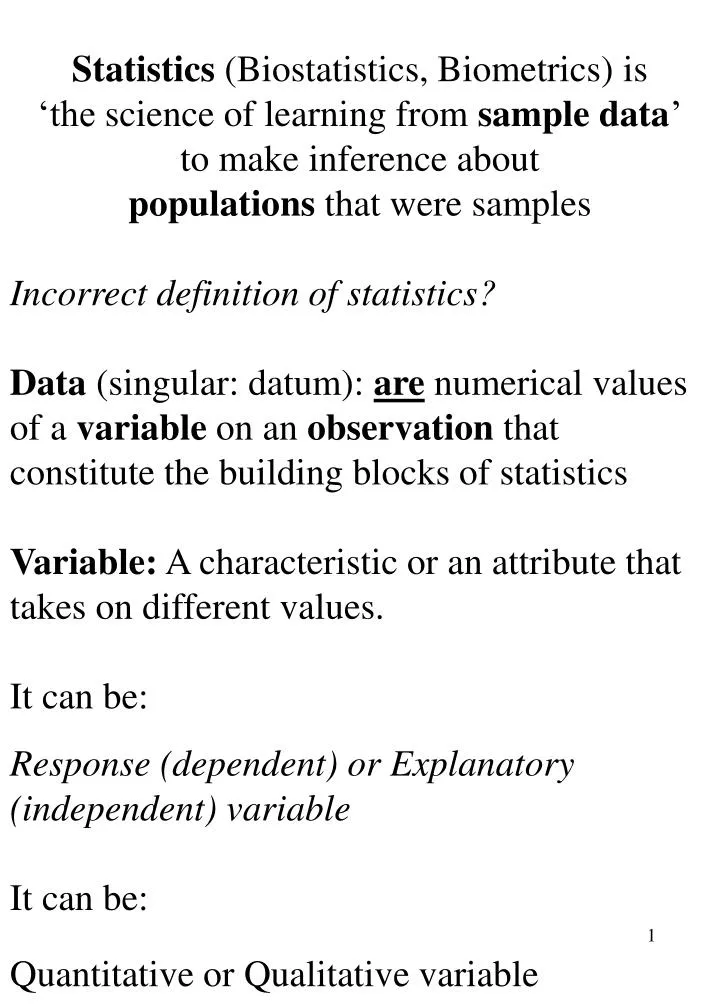
Statistics (Biostatistics, Biometrics) is ‘the science of learning from sample data ’ to make inference about populations that were samples Incorrect definition of statistics?

E N D
Statistics (Biostatistics, Biometrics) is ‘the science of learning from sample data’ to make inference about populations that were samples Incorrect definition of statistics? Data(singular: datum): are numerical values of a variable on an observation that constitute the building blocks of statistics Variable: A characteristic or an attribute that takes on different values. It can be: Response (dependent) or Explanatory (independent) variable It can be: Quantitative or Qualitative variable
Recognition of the kinds of variables is crucial in choosing appropriate statistical analysis Examples of Response and Explanatory variables (when appropriate)? Examples of quantitative and qualitative variables?
Quantitative variables:Convey amount 1. Discrete (counts--frequencies): number of patients, species - there are gaps in the values (zero or positive integers) 2. Continuous (measurements): a. ratio (with a natural zero origin: mass, height, age, income, etc.) b. interval (no natural zero origin: calendar dates, ºF or ºC, etc.) - no gaps in the values - measuring precision is limited by the precision of the measuring device which results in recording it as discrete
Qualitative (categorical) variables:Convey attributes, cannot be measured in the usual sense but can be categorized 1. Nominal: mutually exclusive and collectively exhaustive (gender, race, religion, etc.) - can be assigned numbers but cannot be ordered 2. Ordinal: categorical differences exist, which can be: - numbered and ordered but the distances between values not equal (cold, cool, warm, hot; low, medium, high; sick, normal, healthy; depressed, normal, happy; etc.) Note: both nominal and ordinal variables are discrete
Source of Data and Type of Research:1. Observational studiesExamples?2. Experimental studiesExamples? FieldMesocosmGreen house LaboratoryRecognition of the kind of the study, and the way the study units are selected and treated are crucial in:- making statistical inference- establishing correlational or causalrelationship
Data can be used to perform:1. Descriptive Statistics2. Statistical Modeling 3. Inferential Statistics--Hypothesis Testing
Inferential Statistics • Inference from one observation to a population • e.g.1, comparing body temperature of one bird with the mean body temp. of a bird species • - test statistics? • a) population parameters are known • b) population parameters not known
Inferential Statistics • Inference from several observations to a population • e.g.2, comparing body temperature of three birds with the mean body temp. of a bird species • - test statistics? • a) population parameters are known • b) population parameters notknown
Inferential Statistics • Comparing two or more sets of observations to test whether or not they belong to different populations • e.g., 3, comparing starting salaries of females and males in several organizations to see if their starting salaries differ • - do we know the populations’ parameters? • - can they be estimated? • - what would be the test statistics? • - what would be the scope of inference? • - why do we need Inferential Statistics to do so?
What do we mean by ‘inference’? • Aninference is a conclusion that patterns in the data are present in some broader context • A statistical inference is the one justified by a probability model linking the data to the broader context
Inference from a sample to its parent population, or from samples to compare their parent populations, can be drawn from observational studies • - such inference is optimally valid if the sampling is random • - results from observational studies cannot be used establish causal relationships,but are still valuable in suggesting hypothesis and the direction of controlled experiments • Inference to draw causal relationships can be drawn from randomized, controlled experiments, and not from observational studies
Statistical inference permitted by study designs (Adapted from Ramsey and Schafer, 2002) Inferences to populations Can be drawn Causal inferences can be drawn
Population (probability) Distribution: • Discrete • 1. Binomial (Bernoulli) • 2. Multinomial: a generalized form of binomial where there are > 2 outcomes • 3. Uniform: similar to Multinomial except that the probability of occurrence is equal • 4. Hypergeometric: similar to binomial except that the probability of occurrence is not constant from trial to trial sampling without replacement—dependent trials) • 5. Poisson: similar to binomial but p is very small and the # of trials (s) is very large such that s.papproaches a constant
Population (probability) Distribution: • Discrete (previous slide) • Continuous • 1. Uniform: similar to the discrete uniform but the # of possible outcomes is infinite • 2. Normal (Gaussian):
Population (probability) Distribution: • Discrete • 1. Binomial (Bernoulli): • a. in a series of trials a variable (x) takes ononly 2 discrete outcomes (probability ofoccurrence --p) • b. trials are independent (sampling with replacement) and constant p from trial to trial (e.g., probability distribution of having 1, 2, or 3 girls in 10 families each with 3 kids) • c. probability of occurrence can be equal or unequal
1. Discrete Binomial Distribution • Probability (p) distribution for the number of smokers in a group of 5 people ( n = 5, p of smoking = 0.2, 0.5, or 0.8) • Tabular presentation • # of smoker(s) p = 0.2 p =0 .5 p = 0.8 0 0.328 0.031 0.000 1 0.410 0.156 0.006 2 0.205 0.312 0.051 3 0.051 0.312 0.205 4 0.006 0.156 0.410 5 0.000 0.031 0.328 • Graphical presentation p = 0.2 p = 0.8 p = 0.5 1 0 5 2 3 4 1 0 5 1 2 3 4 0 5 2 3 4 # of smokers
3. Discrete Uniform DistributionProbability (p) distribution for one toss of a die • Tabular presentation • toss p • 1 1/6 • 2 1/6 • 3 1/6 • 4 1/6 • 5 1/6 • 6 1/6 • Graphical presentation p 1/6 1 2 3 4 5 6 toss
Continuous • 1. Uniform • 2. Normal (Gaussian): A bell-shaped symmetric distribution
The Normal distribution is central to the theory and practice of parametric inferential statistics because Distributions of many biological and environmental variables are approximately normal When the sample size (# of independent trials) is large, or p and q are similar, other distributions such as Binomial and Poisson distributions can be approximated by the Normal Dist. The distribution of the means of samples taken from a population i. is normal when samples are taken from a normal population ii. approaches normality as the size of samples (n) taken from non-normal populations increases (Central Limit Theorem--CLT) - implication of CLT?
The normal distribution is a mathematical function (may you observe it in real life??) defined by the following equation:Y = 1 / ( 2) e - (Xi - m)2 / 22, where: X Y : height of the curve for a given Xie : 2.718 : 3.142 m: arithmetic mean, measure of central tendency : measure of the dispersion (variability) of the observations around the meanThe last two characteristics are the two unkownparametersthat shape the distribution
m:the mean, a measure of central tendency - calculated as the arithmetic average - is a parameter - is constant - does not indicate the variability within a population, -when not known, estimated by (a statistic) from unbiased sample(s)
s2: Variance, a measure of variability (dispersion) calculated as: ( y i- m) 2 / N(definition formula) or [ y i2–( yi)2/N ] / N (calculation formula) - its unit is the squared unit of the variable of interest - also called mean square of error (why?) - estimated best by S 2 (a statistic) from unbiasedsample(s) calculated as: ( y i-) 2 / (n-1) or [ y i2-( yi)2/n ] / (n-1) -- what do we call [ y i2-( yi)2/ n ]? • -- is it a good measure of variability? • -- what do we call ‘n-1’? • So, S2 =SS / df • (reason to call it ………………….. – MSe)
- to get a measure of variability in the unit of the variable of interest , we take the square root of the variance and call it Standard Deviation -- is denoted by s (a parameter) for a population, estimated best by S or SD (a statistic) from unbiased sample(s) -- it is a rough (not exact) measure of averageabsolute deviations from the mean
Important properties of a normal distribution: • Because the normal distribution is symmetric characterized by a mean mand a standard deviation of s the followings are true: • a. the total area under the normal curve is 1 or 100% • b. half of the population (50%) is greater and half (50%) is smaller than m • c. 68.27% of the observations are withinm 1s • d. 95.44% of the observations are withinm 2s • e. 99.74% of the observations are withinm 3s • - what do above statements mean in terms of probability (e.g., probabilistic status of one observation falling on the mean, on any boundaries, or anywhere within or outside a boundary)?
Standard Normal Distribution Is the distribution of the Z values where: Z = (Xi - m) / s How many Normal Distributions you may find? How many Standard Normal Distributions you may find? What are the properties of the Standard Normal Distribution? A Ztable in a stat book shows the proportion of the population beyond the calculated Z value
To study populations, it is usually not feasible to measure the entire populationof N members. Why not sampling the entire population? Real (finite and infinite) and Imaginary populations?
Therefore, we draw sample(s) to represent the parent populations Sample is a subset of a population, drawn and analyzed to infer conclusions regarding the population. Its size is usually denoted by n. Sampling can be done: 1. With replacement 2. Without replacement (the norm in practice)
To infer valid (unbiased) conclusions regarding a population from a sample, the sample must represent the entire population. • For a sample to represent the entire population, it is best to be drawn RANDOMLY. • A sample is random when each and every member of the population has an equal and independent chance of being sampled (exceptions?). • Random sampling, on average: • - represents the parent population • - prevents known and unknown biases to affect the selection of observations, and thus, • - allows the application of the laws of probability in drawing a statistical inferences
Descriptive Statistics • Data organization, summarization and presentation • 1. Tabular (tally, simple, relative, relative-cumulative, and cumulative frequencies) • 2. Graphical (histograms, polygons) Suppose we have the following random sample of creativity scores: Case Score Case Score 1 26.7 13 29.7 2 12.0 14 20.5 3 24.0 15 12.0 4 13.6 16 20.6 5 16.6 17 17.2 6 24.3 18 21.3 7 17.5 19 12.9 8 18.2 20 21.6 9 19.1 21 19.8 10 19.3 22 22.1 11 23.1 23 22.6 12 20.3 24 19.8
Steps in data organization, summarization and presentation (Geng and Hills, 1985)1. Determine the range (R): largest - smallest , R = 29.7 - 12 = 17.72. Determine the number of classes (k) into which data are to be grouped a. 8 - 20 classes is often recommended - too few--information loss - too many--too expensive (time, etc.) b. can be calculated based on Sturges’ rule as: k = 1 + 3.3 log n, where n = number of cases, in our case 1 + (3.3)(log 24) = 5.55, and thus k should be at least 6, and this is what we use
Steps in data organization, summarization and presentation (Geng and Hills, 1985)3. Select a class interval (difference between upper and lower class boundaries--R/k may be used, we use 3)4. Select the lower boundary of the lowest class and add the interval successively to it until all data are classified - to avoid falling of data on the boundaries, they are usually expressed to half unit greater than the measurement accuracy - in our case measurement accuracy is 0.1 and so the class boundaries would for example be expressed as 11.05-14.05.5. Arrange the table as follows:
Tallied Relative Class Bound- Mid- Simple Cum. Rel. Cum. point aries freq. freq. freq. freq. freq. 11.55-14.55 13.05 0.167 0.167 4 1 4 IIII 16.05 0.125 0.292 7 2 14.55-17.55 III 3 17.55-20.55 19.05 0.625 15 3 8 0.333 IIIIIIII 22.05 0.292 0.917 22 4 20.55-23.55 7 IIIIIII 0.958 0.042 25.05 23 5 23.55-26.55 I 1 28.05 0.042 1.000 24 6 26.55-29.55 I 1
Stem-and-Leaf DiagramA cross between a table and a graph 12 0 0 9 13 6 14 15 26 6 17 2 5 18 2 19 1 3 8 20 3 5 6 21 3 6 22 1 2 6 23 1 24 0 3 25 26 7 27 28 29 7
Steps in Creating Stem-and-Leaf Diagram 1. Arrange the data in increasing order 2. First, write the whole numbers as the stem 3. Then, write the numbers after decimals, in increasing order, as leaves Advantages: 1. Ease of construction 2. Depiction of individual numbers, min., max., range, median, and mode 3. Depiction of center, spread, and shape of distribution Disadvantages: 1. Difficulty in comparing distributions when they have a very different ranges 2. Difficulty in comprehension and construction when the sample size is very large
Measures of a Dataset that are Important in Descriptive / Inferential Statistics 1. Measure of Central Location (Tendency) 1.1. Mode: the value with highest frequency - there may be no mode, one mode, or several modes - not influenced by extremes - cannot be involved in algebraic manipulation - not very informative 1.2. Median: the middle value when data are arranged in order of magnitude - not influenced by extremes (i.e., useful in economics when extremes should be disregarded - not involved in algebraic manipulation - if n is odd, is the middle value when data are ordered - if n is even, is the average of the two middle values when data are ordered
1.3.Mean: arithmetic average, denoted by: a.m = ( Xi / N): a parameter,for a population, which is best estimated by: b.x : a statistic,from a sample or samples - most frequently used in statistics and subject of algebraic manipulation - is the best estimate of m if the sample is unbiased (representative of its population); the sample is unbiased if it is drawn randomly, not otherwise - the mode, the median, and the mean are the same when the distribution is perfectly symmetrical - the units for the mode, median, and the mean are the same as the unit of the variable of interest - the mean does not indicate the variability of a dataset; e.g., consider the following three sets of data with a common mean: 22, 24, 26 20, 24, 28 16, 24, 32
2. Measure of variability--dispersion 2.1. Range: the largest value - the smallest value (R) - not very informative, often affected by extremes 2.2. Variance (mean square*), represented by two symbols [s 2, sigma square(d), and S 2]: a. s 2: represents the variance of a population;it is a parameter, constant for a given population, quantified as the sum of the squared deviations of individual members from their mean divided by the population size (finite): s 2 = [(X1 - m)2 + (X2 - m)2 + … + (XN - m)2] / N = (Xi - m)2 / N s 2 is estimated best by:
2.2.b.S 2: thevariance ofasample; it is astatistic, which varies from sample to sample taken from a given population, and is calculated as the sum of the squared differences between the sampled individuals and their mean divided by the sample size minus one: S 2= (xi- x) 2 / n-1, which is the definition formula and can be reduced to a computation formula as: S 2= [xi2-(xi) 2 / n ] / n-1 - easier to calculate - scientific calculators provide the components - more accurate because no rounding of numbers is involved
Notes: - S2 is the best estimate of s 2 if the sample is unbiased (representative of its population); the sample is unbiased if it is drawn randomly, not otherwise - the unit of the variance is the square of the unit of the variable of interest - the quantity “xi2-(xi) 2 / n” is calledsum of squaresorSS, it is aminimum - the quantity “(xi) 2 / n”is calledthecorrection factor or C -the quantity “n-1” is called degrees of freedom or df - Thus, Variance = sum of squares / degrees of freedom, or S2 =SS / df * this is why the variance also is called “mean square”
2.3. Standard Deviation: square root of the Variance a. s : aparameter,for a population: b. S or SD: astatistic, for a sample - unit of standard deviation is the same as that of the variable of interest 2.4. Coefficient of Variation (CV ): is a relative term (%) - calculated as (SD / x ) × 100 - used to compare the results of several studies done differently (different experimenters, procedures, etc.) on the same variable
2.5. Skewness: measure of deviationsfromsymmetry a. symmetrical (skewness = 0) b. Skewed to the left (skewness > 0) c. skewed to the right (skewness < 0) 2.6. Kurtosis : measure of peakedness or tailedness a. mesokurtic (kurtosis = 0) b. leptokurtic (kurtosis > 0) c. platykurtic (kurtosis < 0)
Sampling Means Distribution • Is the distribution of the means of all possible samplesof size n taken from a population. • If sampled from a normal distribution will be normal • If sampled from a non-normal dist. becomes more normalthan the parent dist. (Central Limit Theorem- CLT*) • - as sample size is increased, the sampling mean distribution approaches normality • *Fuzzy CLT: • Data influenced by many small, unrelated, random effects are approximately normally distributed.
The sampling mean distribution has a: • - mean, equal to m (mean of population) • - variance (measuring average squared deviation of the sampled means from m), • -- calculated as variance of the means, or s2/n (based on LLN) • -- estimated best by S2 /n • - - denoted as or , respectively • -- square root of the above variance • is called ………………………… or …………..…………….. • or …………..……………..
Standard Error: • Is a rough measure of the average absolute • deviation of sampling meansfrom m (typical • error made when estimating m from themean of a sample of size n) • can be calculated as: s / n • best estimated by S / n • denoted as or orSE