Chapter 3 Image Enhancement in the Spatial Domain

1. Chapter 3Image Enhancement in the Spatial Domain 國立雲林科技大學 資訊工程所 張傳育(Chuan-Yu Chang ) 博士 Office: EB212 TEL: 05-5342601 ext. 4337 E-mail: chuanyu@yuntech.edu.tw Website:MIPL.yuntech.edu.tw

2. Preview • The principal objective of enhancement is to process an image so that the result is more suitable than the original image for a specific application. • Image enhancement approaches • Spatial domain methods • Based on direct manipulation of pixels in an image. • Frequency domain methods • Based on modifying the Fourier transform of an image.

3. Background • Spatial domain • Refers to the aggregate of pixels composing an image. • Operate directly on these pixels Spatial domain process willbe denoted by g(x,y)=T[f(x,y)] where f(x,y): input image g(x,y): processed image T: an operator mask filter kernel template windows

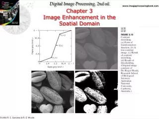
4. Background (cont.) • Gray-Level (intensity) transformation Function • s=T(r) • where T is gray-level transformation function • Processing technologies: • Point processing • Enhancement at any point in an image depends only on the gray level at that point. • Mask processing or filtering • Use a function of the values of f in a predefined neighborhood of (x,y) to determine the value of g at (x,y) Contrast stretching thresholding

5. Some Basic Gray Level Transforms • Some basic Gray Level Transforms • s = T(r) • r : the gray level value before process • s: the gray level value after process • Values of the transformation function typically are stored in a one-dimensional array and the mapping from r tos are implemented via table lookups.

6. Some Basic Gray Level Transforms (cont.) • Image Negatives • Reversing the intensity levels of an image • Photographic Negative • s=L-1-r • Suited for enhancing white or gray detail embedded in dark regions of an image

7. Some Basic Gray Level Transforms (cont.) • Log Transformations • s=c log (1+r) • Maps a narrow range of low gray-level values in the input image into a wider range of output levels. • To expand the values of dark pixels in an image while compressing the higher-level values A Fourier spectrum with values in the range 0 to 1.5x106. c=1, the range of values : 0 to 6.2.

8. Some Basic Gray Level Transforms (cont.) • Power-Law Transformations • s=crg • s= c (r +e)r • wherec and `g are positive constants • Power-law curves with fractional values of r map a narrow range of dark input values into a wider range of output values, with the opposite being true for higher values of input levels. To account for an offset

9. Some Basic Gray Level Transforms (cont.) • Gamma Correction • The process used to correct this power-law response phenomena

10. Fracture dislocation Some Basic Gray Level Transforms (cont.) c=1, g=0.6 • Example 3.1 • MR image of fractured human spine • Contrast manipulation c=1, g=0.4 c=1, g=0.3 The best enhancementin terms of contrast and discernable detail wasobtained. 褪色(Washed-out)

11. Some Basic Gray Level Transforms (cont.) c=1, g=3.0 c=1, g=5.0 Washed-out appearance c=1, g=4.0

12. Some Basic Gray Level Transforms (cont.) Picewise-Linear Transformation Function • Contrast Stretching • To increase the dynamic range of the gray levels in the image being processed. • Linear function • Ifr1=s1 and r2=s2 • Thresholding • If r1=r2, s1=0 and s2=L-1 Control points

13. Some Basic Gray Level Transforms (cont.) Picewise-Linear Transformation Function • Gray-level Slicing • Highlighting a specific range of gray levels in an image. • To display a high value for all gray levels in the range of interest and a low value for all other gray levels. • Brightens the desired range of gray levels but preserves the background and gray-level in the image.

14. Some Basic Gray Level Transforms (cont.) • Bit-plane Slicing • Highlighting the contribution made to total image appearance by specific bits. • Separating a digital image into its bit planes is useful for analyzing the relative importance played each bit of the image. • Determining the adequacy of the number of bits used to quantize each pixel. • Image compression.

15. Some Basic Gray Level Transforms (cont.) • An 8-bit fractal image

16. Some Basic Gray Level Transforms (cont.) • The eight bit planes of the image in Fig. 3.13

17. Histogram Processing Histogram h(rk)= nk rkis thekth gray-level nkis the number of pixels in the image having gray-levelk Normalized Histogram p(rk)=nk/n

18. Histogram Processing (cont.) • Histogram Equalization Assume that the transformation functionT(r)satisfies the follows (a) T(r)is a single-valued and monotonically increasing (b) 0<=T(r)<=1 for 0<=r <=1

19. Histogram Processing (cont.) • The probability of occurrence of gray level rk in an image is approximated by • The discrete version of the transformation function given as • A processed image is obtained by mapping each pixel with level rk in the input image into a corresponding pixel with level sk in the output image. Histogram equalization automatically determines a transformation function that seeks to produce an output image that has a uniform histogram.

20. Histogram Processing (cont.) • Example 3.3Histogram equalization

21. Histogram Processing (cont.)

22. Histogram Processing (cont.) • Histogram matching (Specification) • Let s be a random variable with the property • Define a random variable z with the property • Assume that G(z)=T(r), therefore, that z must satisfy the condition (3.3-10) (3.3-11) (3.3-12)

23. Histogram Processing (cont.) • Histogram matching (Specification) • To specify the shape of the histogram that we wish the processed image to have. (3.3-13) (3.3-14) (3.3-15) (3.3-16)

24. Histogram Processing (cont.) 1.對原圖進行histogram equalization 2.對給予的histogram,計算轉換函數G(z) 根據手繪函數G(z)求出每個Zq所對應的vq 3.對每個sk，求對應的Zk

25. Procedure for histogram matching • Obtain the histogram of the given image • Use E.q.(3.3-13) to precompute a mapped level sk for each level rk • Obtain the transformation function G(z) from the given pz(z) using Eq.(3.3-14) • Precompute zk for each value of sk using the scheme defined in Eq(3.3-17) • Use the value from step (2) and step (4), mapping rk to its corresponding level sk, then map level sk into the final level zk.

26. Histogram Processing (cont.) • Example 3.4 Comparison between histogram equalization and histogram matching 火星的衛星影像，有大區域的深色區域，由其histogram觀察， 會以為histogram equalization會有不錯的結果？

27. Histogram Processing (cont.) 由於圖3.20中的histogram,gray level 0及其附近有大量的值，因此根據Eq(3.3-8)，s0會接近190。 直接以圖(a)進行equalization會有褪色的感覺。

28. Histogram Processing (cont.) 轉換後的結果 手繪的histogram 手繪的histogram之 轉換函數G(z) 轉換後的histogram

29. Local Enhancement • Global enhancement • The pixels are modified by a transformation function based on the gray-level content of an entire image. • Local enhancement • To design transformation functions based on the gray-level distribution in the neighborhood of every pixel in the image. • Local enhancement Procedure • Step 1: Define a square neighborhood • Step 2: Move the center of this area from pixel by pixel • Calculate the histogram of the points in the neighborhood. • Apply the histogram equalization or specification • Assign new gray level to the center pixel • Step 3: Moved to an adjacent pixel location. • Repeat Step 2 until end of the image

30. Histogram Processing (cont.) • Example 3.5 • Enhancement using local histograms Result of local histogram equalization Result of global histogram equalization Original image

31. Use of Histogram Statistics for Image Enhancement • The global mean and variance • The mean is a measure of average gray level in an image • The variance is a measure of average contrast in an image. • Let r denote discrete gray-levels in the range • p(ri) denote the normalized histogram component corresponding to the ith value of r. • The nth moment of r is defined aswhere m is the mean value of r (3.3-18) (3.3-19)

32. Use of Histogram Statistics for Image Enhancement • 根據(3.3-18)及(3.3-19)m0=1, m1=0 • The second moment is obtained by • (3.3-20)為r的variance。 • Standard deviation定義為variance的平方根(square root) 。 • The global mean and variance are measured over an entire image and are useful primarily gross adjustments of overall intensity and contrast. (3.3-20)

33. Histogram Statistics for Image Enhancement • The local mean and variance • The local mean is a measure of average gray level in neighborhood Sxy • The variance is a measure of contrast in the neighborhood (3.3-21) (3.3-22)

34. Example 3.6 鎢絲1(清楚) 鎢絲2(不清楚)

35. Example 3.6 • The problem is to enhance dark areas while leaving the light area as unchanged as possible. • Consider the pixel as a point (x,y) as a candidate for processing

36. Histogram Processing (cont.) 對影像取localmean average 對影像取localstandard deviation 三個條件判別 後的結果 白色部分為 E，用來對原影像相乘，以得到強化的結果。 採用3x3 local region

37. Histogram Processing (cont.)

38. Enhancement using Arithmetic/Logic Operations • Enhancement using Arithmetic/Logic Operations • Arithmetic/Logic operations are performed on a pixel-by-pixel basis. • Arithmetic operations: subtraction, addition, division, multiplication. • Logic operations: AND, OR, NOT • When dealing with logic operations on gray-scale images, pixel values are processed as strings of binary numbers.

39. Enhancement using Arithmetic/Logic Operations (cont.)

40. Enhancement using Arithmetic/Logic Operations (cont.)

41. Enhancement using Arithmetic/Logic Operations (cont.) • Image Subtraction • The enhancement of difference between images • The difference between two images f(x,y) and h(x,y) (3.4-1)

42. Enhancement using Arithmetic/Logic Operations (cont.) • Most images are displayed using 8 bits. • Thus, we expect image values not to be outside the range from 0 to 255. • The value in a difference image can range from a minimum of -255 to a maximum of 255. • How to solve this problem? • Solution 1: g’(x,y)=[g(x,y)+255]/2 • Solution 2:g’(x,y)=g(x.y)-min(g(x,y))g’’(x,y)=[g’(x,y)*255]/max(g’(x,y))

43. Enhancement using Arithmetic Operations (cont.) • Image averaging • Noisy image g(x,y)formed by the addition of noise h(x,y) to an original image f(x,y)Assume that at every pair of coordinates (x,y) the noise is uncorrelated and has zero average value. • Averaging K different noisy images • To reduce the noise content by adding a set of noisy images • The standard deviation at any point in the average image is (3.4-2) (3.4-3) (3.4-6) As K increases, Eq(3.4-6) indicates that the noise of the pixel values at each location (x,y) decreases.

44. Enhancement using Arithmetic/Logic Operations (cont.) • Example 3.8 Noise reduction by image averaging • The images gi(x,y) must be registered in order to avoid the introduction of blurring and other artifacts. • (a) Image of Galaxy pair NGC 3314. • (b) Image corrupted by additive Gaussian noise with zero mean and a standard deviation of 64 gray levels. • (c-f) Result of averaging K=8, 16, 64 and 128 noisy images.

45. Enhancement using Arithmetic/Logic Operations (cont.) In the histograms, the mean and standard deviation of the difference images decrease as K increases.

46. Basic of spatial filtering • Basic of spatial filtering If image size M×N, mask size m×n where a=(m-1)/2 b=(n-1)/2 Convolving a mask with an image

47. Basic of spatial filtering (cont.)

48. Smoothing Spatial Filter • Smoothing filters are used for blurring and for noise reduction. • Smoothing Linear Filter • Sometimes are called averaging filter , lowpass filter • Box filter • A spatial averaging filter in which all coefficients are equal • Weighted average • Pixels are multiplied at different coefficient

49. Smoothing Spatial Filter (cont.) • Example 3.9 • Image smoothing with masks of various sizes • (a) Original image of size 500x500 • (b-f) Results of smoothing with square averaging filter masks of sizes n=3, 5, 9, 15, and 35.

50. Smoothing Spatial Filter (cont.) • Spatial averaging is to blur an image for the purpose getting a gross representation of objects of interest. • The intensity of smaller objects blends with the background and larger objects become “bloblike” and easy to detect.