Wavevector (Phase) Matching

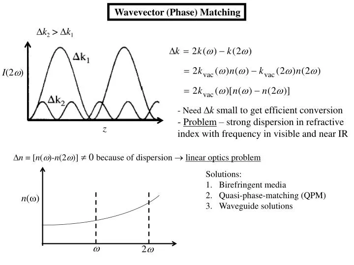
1. k2 > k1 n() I(2)  2 z Wavevector (Phase) Matching • Need k small to get efficient conversion • - Problem – strong dispersion in refractive index with frequency in visible and near IR n = [n()-n(2)]  0 because of dispersion linear optics problem • Solutions: • Birefringent media • Quasi-phase-matching (QPM) • Waveguide solutions

2. x - optically isotropic in the x-y plane - z-axis is the “optic axis” - for , any two orthogonal directions are equivalent eigenmode axes  cannot phase-match for z y BirefringentPhase-Matching: Uniaxial Crystals in x-z plane, ne() • - Note: all orthogonal axes in x-y plane • are equivalent for linear optics • always in x-y plane • always has z component • - angle from x-axis important for x in x-z plane Uniaxial Crystals  y = 0 z along y-axis, no Convention: “ordinary” refractive index “extraordinary” refractive index

3. E E e e E o ne no Type I Phase-Match 1 fundamental eigenmode 1 harmonic eigenmode +veuniaxialoee +veuniaxial  ne>no no(2) = ne(,) Harmonic (1 photon) Fundamental (need 2 identical photons) k = 2ke()– ko(2) = 2kvac()[ne(,)-no(2] x x y y z z E o Critical phase-match 0<</2 Non-critical phase-match =/2 no(2) = ne(,) no(2) = ne() n() n() ne no ne(,)

4. Because of optical isotropy in x-y plane for phase-matching lies on a cone at an angle from the z-axis lies in x-y plane Note: does depend on angle  from x-axis in x-y plane!! Range of phase-match frequencies limited by condition ne() no(2)

5. Non-critical phase-match =/2 no() = ne(,2) -veuniaxialeoo Harmonic Fundamental no ne Type I -veuniaxial  no>ne k = 2ko()– ke(2) = 2kvac()[no()-ne(,2] Critical phase-match 0<</2 n() n() ne() no ne

6. Type II Phase-Match 2 fundamental eigenmodes 1 harmonic eigenmode +veuniaxial  ne > no +veuniaxialoeo Fundamentals, need 2 (orthogonally polarized) photons Harmonic (1 photon) k = ke() + ko() –ko(2) = kvac(){[ne(,)+no()] - 2no(2)} n() ne no

7. Type II -ve uniaxial  no> ne -veuniaxialeoe Harmonic Fundamental k = ke() + ko() –ke(2)= kvac()[ne(,) + no()] - kvac(2)ne(,2) = kvac(){[ne(,) + no()] - 2ne(,2)} n() no Unique  ne

8. “Non-Critical” Phase Match “Critical” Phase Match Z (optic) axis Type I eoo PM ne(2,) no(2) Poynting vectors no() = ne(2) Curves are tangent no() Difference between the normals to the curves represent spatial walk-off between fundamental and harmonic Reduces conversion efficiency ne(,)

9. “Critical” Versus “Non-Critical” Phase Match How precise must PM be? I(2)  sinc2[kL/2= /2]  4/2 0.5 e.g. Type I eoo (-veuniaxial) I(2,) 0 PM (Half width at half maximum) Usually quote the “full” acceptance angle = 2PM  Note key role of birefringence

10. Small birefringence is an advantage in maintaining a useful angular bandwidth Non-collinear Phase-Matching We have discussed only collinear wavevector matching. However, clearly it is possible to extend the wavelength range of birefringent phase-matching by tilting the beams. Interaction limited to this region Biggest disadvantage: Walk-off

11.  z x p’th Fourier component Quasi-Phase-Matching - direction of is periodically reversed along a ferroelectric crystal a is the “mark-space ratio” Periodically poled LiNbO3(PPLN): 1a>0 PPLN k = 2ke() – ke(2) + pK Change phase-matching condition by manufacturing different 

12.  x A – perfect phase match with B – QPM with p=1 n() n(2) C - Quasi-Phase-Matching: Properties (1) c/ z A modified form of “non-critical” phase-match

13. Not useful since Not useful because Phase matching is possible • Higher order gratings can be used to extend phase-matching to shorter wavelengths, although the nonlinearity does drop off, Quasi-Phase-Matching: Properties (2) k = 2ke() – ke(2) + pK The relative strengths of the Fourier components depend on a.

14. State-of-the-art QPM LiNbO3 • fundamental and harmonic co-polarized • d(2)eff  16 pm/V (p=1) • samples up to 8 cms long • conversion efficiency  1000%/W (waveguides) • commercially available from many sources • still some damage issues Right-hand side picture shows blue, green-yellow and red beams obtained by doubling 0.82, 1.06 and 1.3 m compact lasers in QPM LiNbO3

15. Solutions to Type 1 SHG Coupled Wave Equations e.g. Type I -first assume negligible fundamental depletion valid to 10% conversion E()  2 E() E(2) E(2) and E() are /2 out of phase at L=0!!! Large Conversion Efficiency (assume energy is conserved  Kleinman limit) Field Normalization

16. Normalized Propagation Distance Normalized Coupling Constant Normalized Wavevector Detuning “Global Phase” Inserting into coupled wave equations and separating into real and imaginary equations Integrated by the method of the variation of the parameters

17. Sgn is determined by the sign of boundary (initial) condition sine( ) The general solution is given in terms of Jacobi elliptic function Solutions simplify for s=0, i.e. on phase-match The conversion efficiency saturates at unity (as expected)

18. k2 > k1 I(2) z Note the different shape of the harmonic response compared to low depletion case Δs0 Δs=0.2 Δs=0.2 The main (Δk=0) peak with increasing input which means that the tuning bandwidth becomes progressively narrower. The side-lobes become progressively narrower and their peaks shift to smaller ΔkL. (solid black line); (dashed black line); (red dashed line); (solid blue line, curve multiplied by factor of 4).

19. Solutions to Type 2 SHG Coupled Wave Equations E1()  2 E3(2)  E2() Normalizations Physically useful solutions are given in terms of the photon fluxes N(), i.e. photons/unit area Simple analytical solutions can only be given for the case Δs=0

20. Type 2 SHG: Phase-Matched • No asymptotic final state • All intensities are periodic • with distance • Oscillation period depends • on input intensities