Download
1 / 22
230 likes | 1.4k Views
Adjusted Exponential Smoothing. Paul Mendenhall BusM 361 Professor Foster. Outline. Tool defined Equation Explained Illustrated step by step problem Practice Problem Summary. Definition. Times Series Forecasting model Adjusts for trends in information. Trends. What are trends?

E N D
Adjusted Exponential Smoothing Paul Mendenhall BusM 361 Professor Foster
Outline • Tool defined • Equation Explained • Illustrated step by step problem • Practice Problem • Summary
Definition • Times Series Forecasting model • Adjusts for trends in information
Trends • What are trends? Long term movements in a time series. • Why are trends a problem? Cause lags in forecasts.
Smoothing and Alpha • Alpha (α) • If randomness is great than α is closer to 0. • More weight on past data. • If randomness is small than α is closer to 1. • Greater weight on recent data.
Why the Model is Used • Smoothes random information. • Works with trends in information. • Provides a more accurate forecast.
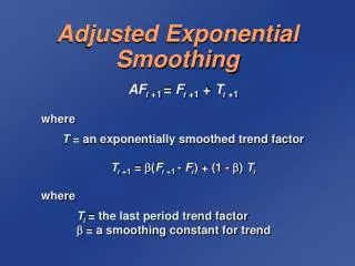
Equation The equation is: AFt+1 = F t+1 + Tt+1
Equation Explained The equation is: AFt+1 = F t+1 + Tt+1 where: F t+1 = αDt + (1- α)Ft T t+1 = β(F t+1 -Ft) + (1- β)Tt Tt=1 = trend factor for the next period. Tt = trend factor for the current period β = smoothing constant for the trend adjustment factor.
Equation Illustrated An electronics company is selling portable CD players and estimated the demand for the first period and forecasted the next three periods' adjusted demand using the Adjusted Exponential Smoothing model. The first periods demand is 50 players and 54 players was used to start the forecast. β = 0.7 and α= 0.2 (see Table 1)
Step 1 • Create a table in Excel and enter the figures for the first period. • Demand was 54. • Unadjusted Forecast is any reasonable starting figure to start the process, in this case 50 players.
Step 2 Calculate Ft+1 for period 2: F t+1 = αDt + (1- α)Ft F2 = 0.2*57+(1-0.2)*50 = 50.8
Step 3 Calculate the trend adjustment factor for period 2: T t+1 = β(F t+1 -Ft) + (1- β)Tt T2 = 0.7(50.8-50)+(1-0.7)*0 = 0.56
Step 4 Calculate the Adjusted Forecast AFt: AFt+1 = F t+1 + Tt+1 AF2 = 50.8 + 0.56 = 51.36
Complete the table Now calculate the Adjusted Forecast for period 3.
Steps 1-4 Completed • Now calculate the Adjusted Forecast for period 3. • Forecast table completed.
Real World Example Concise Co. is considering purchasing new equipment to improve productivity, but must first do some financial analysis. To provide accurate information for the analysis, an accurate forecast of demand must be produced to determine the estimated profit and cash flows for the next year. Concise Co. is concerned about the accuracy of the forecast due to dramatic movements is demand the last few years. Top management has asked you, the financial analysis, to create the forecasted report for 2005.
Real World Ex. Continued You decide, after looking at the trends of the information, that the adjusted exponential smoothing model would work best for the forecast. Alpha is .3 and beta is .6. Use the last five years to create next year’s forecasted demand…
Real World Ex. Continued Top management has asked you, the financial analysis, to create the forecasted report for 2005. Use the last five years to create next year’s forecasted demand. The last five years demand is provided in the graph below.
Summary • Times series • Smoothing • Trends • Accurate forecasting
Additional Readings • http://www.duke.edu/~rnau/411outbd.htm • “Introduction to Operations and Supply Chain Management” Bozarth, Cecil C., Handfield, Robert B. 1st ed. 2005