Download
1 / 14
150 likes | 545 Views
Forecasting Exponential Smoothing For Stationary Models. Exponential Smoothing. The Last Period method uses only one period (the last) and the n-Period Moving Average and Weighted Moving methods use only the last n periods to make forecasts – the rest of the data is ignored .

E N D
Forecasting Exponential Smoothing For Stationary Models
Exponential Smoothing • The Last Period method uses only one period (the last) and the n-Period Moving Average and Weighted Moving methods use only the last n periods to make forecasts – the rest of the data is ignored. • Exponential Smoothingusesall the time series values to generate a forecast with lesser weights given to the observations further back in time.
Basic Concept Weight placed on last estimate for the Level Revised Estimate of the Level at time t Last estimate for the Level Weight placed on current time series value Current time series value • Exponential smoothing is actually a way of “smoothing” out the data by eliminating much of the “noise” (random effects). • At each period t, an exponentially smoothed level, Lt, is calculated which updates the previous level, Lt-1, as the best current estimate of the unknown constant level, β0, of the time series by the following formula: Lt = αyt + (1-α)Lt-1
α in Exponential Smoothing • The idea behind “smoothing” the data is to get a more realistic idea about what is “really going on”. • The value of the smoothing constant, α, is selected by the modeler. • Higher values of α allow the time series to be swayed quickly by the most recent observation. • Lower values keep the smoothed time series “flatter” as not that much weight will be given to the most recent observation. • Usual values of α are between about .1 and .7 • See graphs for α = .1 and α = .7 later in this module. • The value (1-α) is called the damping factor.
Using Exponential Smoothing to Prepare Forecasts in Stationary Models • The Level, Lt, calculated at time period t is the best estimate at time t for the unknown constant, β0. • Since that is the best estimate of β0, it will be the forecast for the next data value of the time series, Ft+1. • Since the model is stationary, it will be the forecast for all future time periods until more time series data is observed. Ft+1 = Lt
Exponential Smoothing Technique • Once a value of α has been selected, the Level (or smoothed value) at time t depends on only two values -- • The current period’s actual value (yt) with weight of a. • The forecast value for the current period (which is the level at the previous period, Lt-1) with weight of 1-a. • Calculations then, for Lt (and hence for Ft+1) are very simple. • Initialization Step – • There is no L0. So we cannot calculate L1 by αy1+ (1-α )L0 • Since y1 is the only value known after period 1, set: Initialization Step L1 = y1
Sample Calculations for First Four Periods of Yoho Data • The first four values of the time series for the Yoho yoyo time series were: 415, 236, 348, 272 • Suppose we have selected to use a smoothing constant of α = .1. Initialization – Period 1 L1 = y1 = 415 -- the level for week 1 is 415 F2 = L1 = 415 -- the forecast for week 2 is 415
Continued Week 2 L2 = .1y2 + .9L1 = .1(236) + .9(415) = 397.1 The smoothed (leveled) value for week 2 is 397.1 F3 = L2 = 397.1 The forecast for week 3 is 397.1 Week 3 L3 = .1y3 + .9L2 = .1(348) + .9(397.1) = 392.19 The smoothed (leveled) value for week 3 is 392.19 F4 = L3 = 392.19 The forecast for week 4 is 392.19 Week 4 L4 = .1y4 + .9L3 = .1(272) + .9(392.19) = 380.171 The smoothed (leveled) value for week 4 is 380.171 F5 = L4 = 380.171 The forecast for week 5 is 380.171
Excel – Exponential Smoothing =.1*B3+.9*C2 =B2 =D54 =C3 Drag D3 down to D54 Drag D55 down to D56 Drag C3 down to C53 Note: Rows 8-43 are hidden
How Exponential Smoothing Uses All Previous Time Series Values • Recall that the recursive formula used is: Lt = αyt + (1-α)Lt-1 • This means: Lt-1 = αyt-1 + (1-α)Lt-2 Lt-2 = αyt-2 + (1-α)Lt-3 Lt-3 = αyt-3 + (1-α)Lt-4 Etc. • Substituting, Lt = αyt + (1-α)Lt-1 = αyt + (1-α)(αyt-1 + (1-α)Lt-2) = = αyt + α(1-α)yt-1 + (1-α)2Lt-2 = = αyt + α(1-α)yt-1 + α(1-α)2yt-2 + (1-α)3Lt-3 = αyt + α(1-α)yt-1 + α(1-α)2yt-2 + α(1-α)3yt-3 + (1-α)4Lt-4 Etc. • Thus all time series values, yt, yt-1, yt-2, yt-3, etc. will be included with successive weights reduced (dampened) by a factor of (1-α).
How Much Smoothing Is There? Exponential Smoothing (α = .1) Actual Data Smoothed time series with α = .1 • We said the lower the value of α, the more “smooth” the time series will become. A “flat” smoothed series
What About Larger Values of α? Exponential Smoothing (α = .7) Actual Data Smoothed time series with α = .7 • Here is the “smoothed” series for α = .7: Very sensitive to most recent time series value – not much smoothing
What Value of α Should Be Used? • Up to the modeler • If the modeler is considering several values of α, a forecast using each value could be prepared. • Only consider values of α that would give useful results (not α = 0, for instance) • Then a performance measure (MSE, MAD, MAPE, LAD) could be used to determine which of the values of α that are being considered have the lowest value of the selected performance measure.
Review • Exponential smoothing is a way to take some of the random effects out of the time series by using all time series values up to the current period. • The smoothed value (Level) at time period t is: α(current value) + (1-α)(last smoothed value) • Forecast for period t+1= Smoothed Value at t • Initialization: First smoothed value = first actual time series value • The smaller the value of α, the less movement in the time series. • Excel approach to exponential smoothing