Download
1 / 32
320 likes | 423 Views
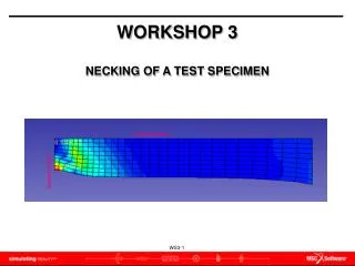
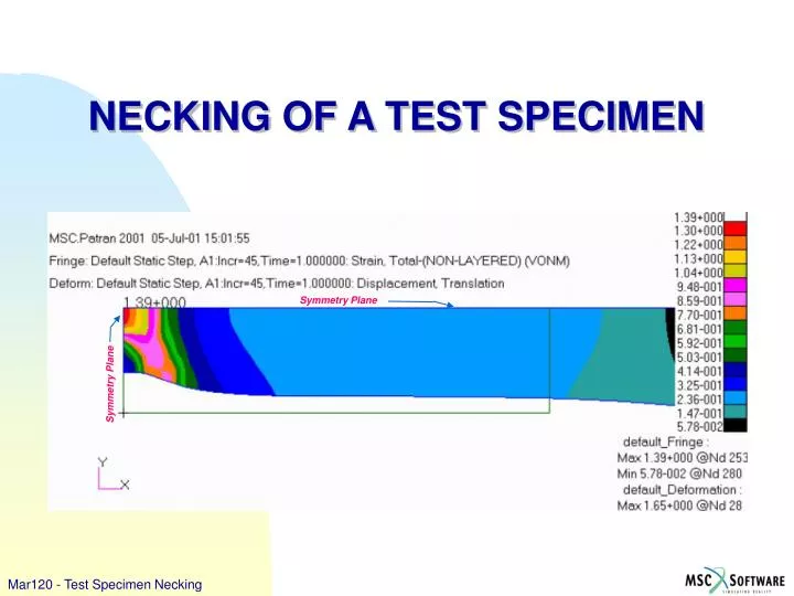
Symmetry Plane. Symmetry Plane. NECKING OF A TEST SPECIMEN. Model Description

E N D
Symmetry Plane Symmetry Plane NECKING OF A TEST SPECIMEN
Model Description • In this lesson, you will stretch an 8 inch long planar steel bar by 1.65 inches (i.e. more than 20% of its length). This elastic-plastic problem will demonstrate the importance of the concept of true stress (or Cauchy stress) in non-linear analysis. This test specimen will be modeled using a quarter symmetry model.
Objective • Large Deflections/Strains analysis • Elastic-Plastic material model using isotropic hardening • Required • No supporting file is required. • Suggested Exercise Steps • Create a 4x1 inch surface in the XY plane Model the contact surfaces with LBC contact • Mesh the model with 16x4 mesh of QUAD/4 elements. • Fix the vertical and horizontal lines of symmetry of the bar and pull the other end by 1.65 inches.
Step 1. Exercise Procedure: File / New a Necking e c b f Necking Create a new database called rubber_seal.db. • File / New. • Enter Necking as the file name. • Click OK. • Wait a few seconds until the New Model Preference opens. • Select MSC.Marc as the Analysis Code. • Click OK.
Step 2. Geometry: Create / Surface / XYZ Geometry: Use the XYZ method to create a 4 x 1 surface. • Geometry: Create / Surface / XYZ. • Enter <4, 1, 0> for the Vector Coordinate List. • Enter [0, 0, 0] for the Origin Coordinate List. • Click Apply. a b <4, 1, 0> c [0, 0, 0] d
Step 3. Elements: Create / Mesh Seed / Uniform a g b c 9 d e Surface 1.1 h f Create Mesh Seeds on the vertical surface. • Elements: Create / Mesh Seeds / Uniform. • Select Number of Elements. • Enter 9 for the Number. • Uncheck Auto Execute. • Click Curve List panel. • Click the Edge picking icon. • Pick the left edge of surface. • Click –Apply-.
Step 4. Elements: Create / Mesh Seeds / One Way Bias a b 27 c 5 d Surface 1.4 g e Create Mesh Seeds on the Horizontal surface. • Create / Mesh Seeds / One Way Bias. • Enter 27 as Number. • Enter 5 as L2/L1. • Click Curve List panel. • Click Edge picking icon. • Pick the bottom edge of surface. • Click –Apply-. f
Step 5. Elements: Create / Mesh / Surface a g 1 1 b c d e Surface 1 h 0.32 i f Mesh the seal. • Create / Mesh / Surface. • Select Quad as the Elem Shape. • Select IsoMesh as the Mesher. • Select Quad4 as the Topology. • Click Surface List panel. • Click Surface or Solid Face. • Pick the surface. • Check Automatic Calculation. • Click –Apply-.
Step 6. Fields: Create / Material Property / Tabular Input a b Plastic_s_e 0 c d e g f The 1D Material Scalar Table Data form needs to be filled out as shown in the table. To fill in the table, click on the cell you wish to edit, enter the value in the Input Scalar Data databox and and press <Return>. The table will automatically tab down. Create a field for the elastic-plastic material data. • Fields: Create / Material Property / Tabular Input. • Enter Plastic_s_e as the Field name. • Uncheck the Temperature (T). • Active Independent Variables: Strain (e). • Click Input Data. • Click OK. • Click –Apply-.
Step 7. Materials: Create / Isotropic / Manual Input d a e 1E7 .33 f * b Mat1 c g h Create the material aluminum_1100, with elastic and plastic properties. • Materials: Create / Isotropic / Manual Input. • Enter Mat1 as the Material Name. • Click Input Properties. • Select Elastic as the Constitutive Model. • Enter 1E7 as the Elastic Modulus. • Enter 0.33 as the Poisson’s Ratio. • Click OK. • Click Apply.
Mat1 Mat1 i n • Click Input Properties. • Select Plastic as the Constitutive Model. • Click the Stress vs Plastic Strain panel. • Click Plastic_s_e. • Click OK. • Click Apply. j Plastic_s_e k l m
o p The Current Constitutive Modelsfor material Mat1 should be two in this exercise: Elastic and Plastic. Do not make the mistake of creating a different Material for each constitutive model.You may define other compatible constitutive models for the same material (Creep for example), not all of which would be used in the same analysis procedure. • Click Mat1. • When you are done inspecting the material, click Cancel.
Step 8. Properties: Create / 2D / 2D Solid a f b Test_specimen c e d g Define the element properties. • Properties: Create / 2D / 2D Solid. • Enter Test_specimen as the Property Set Name. • Select Plane Stress and Standard Formulation as the Option(s). • Click Input Properties. • Select Mat1 as the Material Name by clicking on it in the Material Property Set. • Enter 1 for the Thickness. • Click OK.
Test_specimen Test_specimen i h Surface 1 j Surface 1 k • Click Select Members Panel. • Select Surface 1 using Surface or face icon. • Click Add. • Click –Apply-. We use a biased mesh –we refine the mesh on the vertical (left) symmetry plane- to improve on the accuracy of the FEM-based analysis without having to use a large number of elements. The area close to that plane is the one that sustains the larger strains and therefore it is better to refine the mesh there
Step 9. Loads/BCs: Create / Displacement / Nodal a 1. d <0, , > b Symmetry_vertical Coord 0 e c f Create the three required Displacement Boundary Conditions. • Loads/BCs: Create / Displacement / Nodal. • Enter Symmetry_vertical as the New Set Name. • Click Input Data. • Enter <0,,> as the Translations. • Click OK. • Click Select Application Region.
i g h Surface 1.1 k Surface 1.1 l j • Select Geometry. • Click inside the Select Geometry Entities panel. • Use Curve or Edge picking icon. • Pick the left edge of surface. • Click Add. • Click OK. • Click –Apply-. Symmetry_vertical Symmetry_vertical m
1. p <1.65, 0, > Symmetry_vertical n Pull_at_end Coord 0 q o r • Enter Pull_at_end as the New Set Name. • Open Input Data. • Enter <1.65,0,> as the Translations. • Click OK. • Open Select Application Region.
v s t Surface 1.3 w Surface 1.3 Symmetry_vertical x Pull_at_end u y • Select Geometry. • Click inside the Select Geometry Entities panel. • Use Curve or Edge picking icon. • Pick the right edge of surface. • Click Add. • Click OK. • Click –Apply-.
1. bb < , 0, > Symmetry_vertical Pull_at_end z Symmetry_horiz Coord 0 cc aa dd • Enter Symmetry_horiz as the New Set Name. • Open Input Data. • Enter <,0,> as the Translations. • Click OK. • Open Select Application Region.
ee Surface 1.2 ff Surface 1.2 ii jj Symmetry_verticalPull_at_end hh Symmetry_horiz gg kk • Select Geometry. • Click inside the Select Geometry Entities panel. • Use Curve or Edge picking icon. • Pick the top edge of surface. • Click Add. • Click OK. • Click –Apply-.
Step 10. Display: Load/BC/Elm.Props a Change display mode: Request plotting of Loads/BCs markers on FEM entities. • Display: Load/BC/Elm.Props. • Check Show on FEM only. • Click Apply. • Click Cancel. After this change in the display behavior, loads and BCs will be displayed on FEM entities regardless the filter (Geometry or FEM) you used to create them. b c d
Step 11. Loads/BCs: Plot Markers a b c d Plot Markers. • Loads/BCs: Plot Markers. • Select Displ_Pull_at_end, Displ_symmetry_horiz and Displ_symmetry_vertical. • Select Default_group. • Click –Apply-.
Step 12. Analysis: Analyze / Entire Model / Full Run Analysis • Analysis: Analyze / Entire Model / Full Run. • Enter Necking_job1 as the Job Name. • Open Translation Parameters. • Open Solver Options. • Check Non_Positive Definite. • Click OK. • Click OK. • Click Apply. a d e f b Necking_job1 c h g
a Necking Necking b Read (Attach) results. • Read Results / Result Entities / Attach. • Click Apply.
Step 14. Results: Create / Quick Plot Post-process results. • Result: Create / Quick Plot • Click Deform Attributes icon. • Select True Scale. • Enter 1.0 for the Scale Factor. • Uncheck Show Undeformed option. a b c d 1.0 e
f g h i j k • Click Select Results. • Select the last result case. • Select Stress, Global System. • Select vonMises as the Quantity. • Select Displacement, Translation. • Click Apply.
A local Maximum of stresses occurs in the transition region area (the absolute maximum is in the bottom leftmost corner). Compare with the distribution of strains (later). This problems is sensitive to the numerics of your computer. If the necking happens somewhere towards the center of the mesh rather than next to the left edge, increase the “Number of Desired Iterations” to 7 (in Analysis:Load Step Creation:Solution Parameters:Iterations) and run the analysis again.(記得把disp與residual同時收斂的選項打勾(即and)才會達到同樣的結果,再不行iteration再設大一點到10)
l m n o p • Select the last result case. • Select Strain, Total. • Select von Mises for the Quantity. • Select Displacement, Translation. • Click Apply.
A local Maximum of stresses occurred in the transition region (unlike for strains below) Why? The strain-stress curve define lesser stresses for the largest strains. Thus the maximum strain (in the center of the neck) does not aligns with the maximum stress.
q t r y u s v w x 24 • Create / Deformation. • Click Select Result icon. • Select all the cases. • Click Animation Option. • Select Global Variable as the Animation Method. • Select Time. • Select 2D from Animation Graphics. • Enter 24 as the Number of Frames. • Select Select Results.
Select Displacement, Translation. • Check Animate. • Click Apply. z aa bb