Download
1 / 42
420 likes | 558 Views
Random variable. Distribution. 200 trials where I flipped the coin 50 times and counted heads. no_of_heads in a trial. or I can describe frequencies in percentages. no_of_ones. or as a cumulative histogram. no_of_ones. which can also be in percentage scale. no_of_ones.

E N D
Random variable Distribution
200 trials where I flipped the coin 50 times and counted heads no_of_heads in a trial
or I can describe frequencies in percentages no_of_ones
or as a cumulative histogram no_of_ones
which can also be in percentage scale no_of_ones
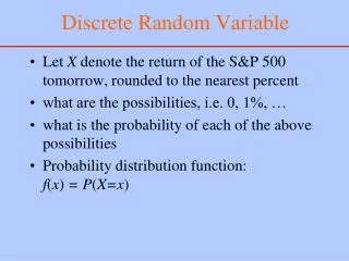
When my population is infinite • Then my number of elements is infinite – but I can characterize it as a proportion from all observations in any interval (i.e. probability, that randomly chosen value in be in interval) • For discrete variable: enumeration of all values and their probabilities pi=P(X=xi) – as a table or formula.
Continuous variable is characterized bydistribution function and probability density probability density Distribution function
Distribution function F(x) =P(X<x) has these basic properties 1. P(a X < b) = F(b) - F(a) ; 2. F(x1) F(x2) pro x1 < x2 ; 3. 4. It is actually idealized cumulative histogram with infinitely narrow columns.
How to “idealize” normal histogram If my columns are endlessly narrow, there will be “nothing” in them – therefore the percentage of observations of the interval is divided by “width” of the column. In a limit case I get for probability density
For distributive function, mean and variance can be computed Discrete variable Continuous variable
Quartile Probability distribution than 12.54 is 75% quantile of distribution (i.e. upper quartile) When this area is 0.75 or 75%
Testing of hypothesis + 2test
I cannot prove any hypothesis • That’s why I formulate null hypothesis (H0), and with rejection of it I prove its opposite. • Alternative hypothesis H1 or HA is negation of the null hypothesis • I, the biologist, am the one who formulates null hypothesis – that’s why null hypothesis would be constructed in such way to be interesting if it is rejected.
Errors in decision • In the case that the data are random (and it is practically every time in biology) I have to take in account that I can make wrong decision – statistics knows Type I error and Type II error, which are unavoidable part of our decision • In addition we can make an error by a mistake in computation, but this isn’t necessary :-) .
Recipe for hypothesis’ testing • 1. I formulate the null hypothesis • 2. I choose the level of significance and so I obtain critical value (from some tables) • 3. I compute test criteria from my data • 4.When the value of test criteria is higher than critical value, I reject the null hypothesis
2test (test of goodness of fit) • Example – I hybridize peas: I expect F1: F2: I have 80 offspring – I expect 60:20, I have 70:10 Is it just random variability, or Mendel’s rates doesn’t work in this case?
1. Rejecting of null hypothesis about 3:1 ratio is interesting from the biological view. I could test statistically null hypothesis about 4,2371:1 ratio, its rejecting doesn’t bring us any biologically interesting information. • 2. Null hypothesis will be in the formal way: probability of dominant phenotype’s manifestation is 0.75 (in infinitely large population of potential offspring is ratio of phenotypes 3:1)
Calculation f - absolutefreqency, i.e. number of random independent observations DF=1 (number of categories - 1 for prior given hypothesis), critical value = 3,84 Value of test criteria > critical value, I reject null hypothesis – I say, ratio in F2is statistically significantly different from expected 3:1 with = 0.05 – or I write (2 = 6.66, df=1, P<0.05)
What can happen – flipping the coin Reality – the coin is OK, i.e. P0=P1=0.5 (BUT WE DON’T KNOW THIS) 100 flips, I get 55:45 Than2=(55-50)2/50+(45-50)2/50 = 1.0 < 3.84. I cannot reject null hypothesis. Right decision.
What can happen – flipping the coin Reality – the coin is OK, i.e. P0=P1=0.5 (BUT WE DON’T KNOW THIS) 100 flips, I get 60:40 Then2=(60-50) 2/50+(40-50) 2/50 = 4.0 > 3.84. I reject null hypothesisonthe 5% level of significance. I have made Type I error(and I gibbet innocent).We know the probability of the error: it is . Level of significance is subjected to the probability of rejecting null hypothesis providing that it is true.
What can happen – flipping the coin Reality – the coin is false, i.e. P0=P1=0.5 (BUT WE DON’T KNOW THIS) 100 flips, I get 60:40 Then2=(60-50) 2/50+(40-50) 2/50 = 4.0 > 3.84. I reject null hypothesis on 5%level of significance. Right decision(and I gibbet blackguard).
What can happen – flipping the coin Reality – the coin is false, i.e. P0=P1=0.5 (BUT WE DON’T KNOW THIS) 100 flips, I get 55:45 Then2=(55-50)2/50+(45-50)2/50 = 1.0 < 3.84. I cannot reject null hypothesis (and blackguard is free). I have committed Type II error. Its probability is signed as and it is mostly unknown. 1 - ispower of the test. Generally, the power of the test is higher with deviation from null hypothesis and with number of observations. As we don’t know, the right formulation of our outcome is: Based on our data we cannot reject null hypothesis. Formulation: We have proved null hypothesisiswrong!
Decision Table Right decision Right decision By given number of observations – the better protected against one type error, the more is outcome predisposed to the second one. If I decide to test on 1% level of significance – the critical value is then 6,63
What can happen – flipping the coin Reality – the coin is OK, i.e. P0=P1=0.5 (BUT WE DON’T KNOW THIS) 100 flips, I get 60:40 Then 2=(60-50) 2/50+(40-50) 2/50 = 4.0 <6,63. I don’t reject null hypothesis on 1% level of significance. - OK, I didn’t gibbet innocent.
What can happen – flipping the coin Reality – the coin is false, i.e. P0=P1=0.5 (BUT WE DON’T KNOW THIS) 100 flips, I get 60:40 Then2=(60-50) 2/50+(40-50) 2/50 = 4.0 < 6,63. I reject null hypothesis on 5% level of significance. Type II error(blackguard is free).
Power of test Reality – the coin is false, i.e. P0=P1=0.5 (BUT WE DON’T KNOW THIS) – When it goes exactly according to probability. 100 flips, I get 55:45 Then2=(55-50)2/50+(45-50)2/50 = 1.0 < 3.84. I don’t reject error II 1000 flips, I get 550:450 Then2=(550-500)2/500+(450-500)2/500 = 10.0 > 3.84. I reject and it is OK. Reality – the coin is false, i.e. P0=0.51; P1=0.49 100 flips, I get 51:49 Then2=(51-50)2/50+(49-50)2/50 = 0.04 < 3.84. I don’t rejecterror II 1000 hodů, dostávám 510:490 Then2=(510-500)2/500+(490-500)2/500 = 0.4 < 3.84. I don’t rejecterror II 10000 flips, I get 5100:4900 Then2=(5100-5000)2/5000+(4900-5000)2/5000 = 4 > 3.84. I reject and it is OK.
Power of test grows • With number of independent observations • With magnitude of deviance from null hypothesis • With lowering protection against Type I error
Percentage of heads in a sample sufficient to reject the null hypothesis P1=P2=0.5 by the 2 -test as a function of totalnumber of observations P<0.01 0.01<P<0.05 P>0.05 percentage P<0.01
Examples of use • phenotype ratio • 3:1 • 9:3:3:1 (number of degrees of freedom = number of categories - 1, for a priori hypothesis, i.e. DF=3)
Examples of use • Sex ratio • 1:1 • Assumptions! • Random sampling! • The same probability In praxis can be rejecting of null hypothesis sign of three facts: 1. Null hypothesis is wrong. 2. Null hypothesis is right, but the decision os consequence of Type I error. 3. Null hypothesis is right, but the assumptions of the test were violated.
Examples of use • Bee’s orientation according to the disk colour • H0: 1:1:1 • How to ensure independence? • Solid size of sample
Examples of use • Hardy-Weiberg’s equilibrium • p2+ 2pq + q • attention – we take off one degree of freedom more for a parameter that we estimate from data, so DF= 3 - 1 - 1 = 1
What are critical values? The higher deviation from null hypothesis, the higher chi-square
What are critical values? When this is 5%, then 11.1 is critical value on 5% level of significance (here is DF=5)
Nowadays is used more often We can use the opposite procedure as well. We have computed chi-square=14 The area of the “tail” = P = 0.014 is “Probability” P is probability, that these or more different result from null hypothesis is just thanks to chance, if H0 is right.
We usually write • the result is significant on = 0.05 - • or we write (2 = 6.66, df=1, P<0.05)
And what is about the 2value is near aroud zero P>0.99 Can we take it as an evidence of true of H0?
2– is deduced just theoretically, but I simulated these values by flipping the coin. Problem - chi-square is continuous distribution, frequencies are discrete from their definition
That’s why Yates` correlation (on continuity) is sometimes used But this test is too conservative then (i.e. probability of error is usually smaller than α, and so the power of test is smaller too). It is not recommended to use, if the expected frequencies > 5, but isn’t used even if just few of them are smaller.