Download
1 / 60
680 likes | 1.08k Views
Successful application of Active Filters. By Thomas Kuehl Senior Applications Engineer and John Caldwell Applications Engineer Precision Analog – Linear Products Texas Instruments – Tucson, Arizona. A filter’s purpose in life. is to…

E N D
Successful application of Active Filters By Thomas Kuehl Senior Applications Engineer and John Caldwell Applications Engineer Precision Analog – Linear Products Texas Instruments – Tucson, Arizona
A filter’s purpose in life is to… Obtain desired amplitude versus frequency characteristics or Introduce a purposeful phase-shift versus frequency response or Introduce a specific time-delay (delay equalizer)
Common filter applications Band limiting filter in a noise reduction application
Common filter applications Delay equalization applied to a band-pass filter application
Filter Types Low-pass High-pass Band-pass Band-stop, or band-reject All-pass Common filters employed in analog electronics
Filter Types Low-pass High-pass fc fc A low-pass filter has a single pass-band up to a cutoff frequency, fc and the bandwidth is equal to fc A high-pass filter has a single stop-band 0<f<fc, and pass-band f >fc Band-stop Band-pass fl fh fl fh A band-stop (band-reject) filter is one with a stop-band fl<f<fh and two pass-bands 0<f<fl and f >fh A band-pass filter has one pass-band, between two cutoff frequencies fl andfh>fl, and two stop-bands 0<f<fland f >fh. The bandwidth = fh-fl
Filter Types An all-pass filter is one that passes all frequencies equally well The phase φ(f) generally is a function of frequency Phase-shift filter (-45º at 1kHz) Time-delay filter (159us)
Filter Ordergain vs. frequency behavior for different low-pass filter orders Pass-band Stop-band fC(-3dB) 1kHz typically, one active filter stage is required for each 2nd-order function
Filter Order 2nd-order low-pass, high-pass and band-pass gain vs. frequency
Filter Responses Response Considerations Amplitude vs. frequency Phase vs. frequency Time delay vs. frequency (group delay) Step and impulse response characteristics
Filter ReponsesCommon active low-pass filters - amplitude vs. frequency Δ attenuation of nearly 30 dB at 1 decade
Filter Reponses – phase and time responses1 kHz, 4th-order low-pass filter example Impulse response Phase vs. frequency Group Delay
Why Active Filters? Inductor size, weight and cost for low frequency LC filters are often prohibitive Magnetic coupling by inductors can be a problem Active filters offer small size, low cost and are comprised of op-amps, resistors and capacitors Active filter R and C values can be scaled to meet electrical or physical size needs A comparison of a 1kHz passive and active 2nd-order, low-pass filter
At fc C1 & C2 impedances are equal to R1 and R2 impedances. Positive feedback is present and Q enhancement occurs Higher Q is attainable with the controlled positive feedback localized to the cutoff frequency Q’s greater than 0.5 are supported allowing for specific filter responses; Butterworth, Chebyshev, Bessel, Gaussian, etc Cascaded 1st-order low-pass RC stages Overall circuit Q is less than 0.5 Q approaches 0.5 when the impedance of the second is much larger than the first; 100x Common filter responses often require stage Qs higher than 0.5 Comparing 2nd-order passive RC and an active filters Resource: Analysis of Sallen-Key Architecture, SLOA024B, July 1999, revised Sept 2002, by James Karki
Two popular single op-amp active filter topologies2nd-order implementations Multiple Feedback (MFB) low-pass • supports common low-pass, high-pass and band-pass filter responses • inverting configuration • 5 passive components + 1 op-amp per stage • low dependency on op-amp ac gain-bandwidth to assure filter response • Q and fnhave low sensitivity to R and C values • maximum Q of 10 for moderate gains Sallen-Key (SK) low-pass • supports common low-pass, high-pass and band-pass filter responses • non-inverting configuration • 4-6 passive components + 1 op-amp per stage • high dependency on op-amp ac gain-bandwidth to assure filter response • Q is sensitive to R and C values • maximum Q approaches 25 for moderate gains
Popular Active Filter Topologies2nd-order implementations Component type for each filter topology
Poles and Zero locations in the s-plane establish the filter gain and phase response third-order low-pass transfer function k H(s) = s3/ω1ω22+ s2(ω1ω2+1/ω22)+s(1/ω1+1/ω2)+1 ω = 2πf, k = gain Transfer function roots plotted in s-plane jω All pole filter responses s = -σ ± jω σ Third-order low-pass transfer function from Burr-Brown, Simplified Design of Active Filters, Function Circuits – Design and Application, 1976, Pg. 228 Response table data from, High Frequency Circuit Design, James K. Hardy, Reston Publishing Company, 1979, table 4A-4, Pg. 152
Complex frequency and active filtersthe s-plane provides the amplitude response of a filter Damping factor (ζ)determines amplitude peaking around the damping frequency fd ζ = cosθ Qthe peaking factor is related to ζ by Q = 1/(2ζ) = 1/(2cos θ) The damping frequency fd is related to the un-damped natural frequency fnby fd= fn (1- ζ2)½ = fn [1- 1/(4Q2)]½ (rect form) fd= fn sin θ (polar form) The pole locations p1, p2 = -ζfn± j fn (1-ζ2)½ s-plane Complex frequency plane Adapted from High Frequency Circuit Design, James K. Hardy, Reston Publishing Company, 1979, Appendix 4A-1, s-PLANE
The damping frequency fd approaches the undamped natural frequency fn as the Q increases fd -3 dB fn Adapted from High Frequency Circuit Design, James K. Hardy, Reston Publishing Company, 1979, Appendix 4A-1, s-PLANE
The stage Q (1/2ζ) affect the time and phaseresponses of the filter Increasing Q higher peaking High Q = longer settling time Decreasing Q - more linear phase change Adapted from Google Images: gnuplot demo script: multiplt.dem
Filter sections are cascaded to produce the intended response the cutoff frequency fc,gain, roll-off, etc is the product of all stages 1 dB Chebyshev, 6th-order LP filter, fc = 10 kHz, Av = 10 v/v • The overall response at Vo is the product of all filter stage responses • Each stage has unique Av, fn, Q • The resulting filter has an fc of 10 kHz, with a pass-band gain of 10 V/V • The 10 kHz pass-band bandwidth is defined by the 1 dB ripple • stage 3 gain was manipulated to be low because of its high Q • Doing so relaxes the GBW requirement – more on this later
Active filter synthesis programsto the rescue! • Modern filter synthesis programs make filter development fast and easy to use; no calculations, tables, or nomograms required • They may provide low-pass, high-pass, band-pass, band-reject and all-pass responses • Active filter synthesis programs such as FilterPro V3.1 and Webench Active Filter Designer (beta) are available for free, from Texas Instruments • All you need to provide are the filter pass-band and stop-band requirements, and gain requirements • The programs automatically determine the filter order required to meet the stop-band requirements • FilterPro provides Sallen-Key (SK), Multiple Feedback (MFB) and differential MFB topologies; the Webench program features the SK and MFB • Commercially available programs such as Filter Wiz Pro provide additional, multi-amplifier topologies suitable for low sensitivity, and/or high-gain, high-Q filters
Operational amplifier gain-bandwidth productan important ac parameter for attaining accurate active filter response
Op-amp gain-bandwidth requirements The active filter’s op-amps should: • Fully support the worst-case, highest frequency, filter section GBW requirements • Have sufficiently high open-loop gain at fn for the worst-case section
The operational-amplifier gain-bandwidth requirements TI’ s FilterPro calculates each filter section’s Gain-Bandwidth Product (GBW) from: GBWsection = G ∙ fn∙ Q ∙ 100 where: G is the section closed-loop gain (V/V) fn is the section natural frequency Q is stage quality factor (Q = 1/2ζ) 100 (40 dB) is a loop gain factor
The operational-amplifier gain-bandwidth requirements Op-amp closed loop gain error • The filter section’s closed-loop gain (ACL) error is a function of the open-loop gain (AOL) at any specified frequency * equivalent noise gain ACL • For example, select AOL to be ≥100∙ACL at fn for ≤1% gain error
The operational-amplifier gain-bandwidth requirement an example of the FilterPro estimation Let FilterPro estimate the minimum GBW for a 5th-order, 10 kHz (fc) low-pass filter having a Chebyshev response, 2 V/V gain and a 3 dB pass-band ripple FilterPro’s GBW estimation for the worst-case stage yields: GBW = G ∙ fn ∙ Q ∙ 100 GBW = (2V/V)(10kHz)(8.82)(100) = 17.64MHz vs. 16.94 MHz from the precise determination – see Appendix for details
Operational amplifier gain-bandwidth effectsthe Sallen-Key topology • The operational amplifier gain-bandwidth (GBW) affects the close-in response • It also affects the ultimate attenuation at high frequency Op-amp fH Hz dB OPA170 90 k -21.8 OPA314 110 k -23.5 OPA340 260k -38.1 OPA140 428 k -44.3 FilterPro GBW 7.1 MHz
Operational amplifier gain-bandwidth effectsthe Multiple Feedback (MFB) topology • The MFB shows much less GBW dependency than the SK • Close-in response shows little effect • Insufficient GBW affects the roll-off at high frequencies • The lowest GBW device (1.2 MHz) produces a gain deviation about 50-60 dB down on the response • A GBW ≥ 7 MHz for this example provides near ideal roll-off
An active filter response issueWhat a customer expected from their micro-power, 50 Hz active low-pass filter (SK) • A customer designed a 50 Hz low-pass filter using the FilterPro software: • Gain = 1 V/V • Butterworth response (Q = 0.71) • The Sallen-Key topology was selected • The FilterPro and TINA-TI simulations using ideal operational amplifiers models produced ideal results • Note FilterPro recommended an operational-amplifier with a gain-bandwidth product (GBW) of 3.55 kHz
An active filter response issueWhat the customer observed with a micro-power, 50 Hz active low-pass filter (SK) • Normal low-pass response below and around the 50 Hz cutoff frequency • The -40 dB/dec roll-off fails about a decade beyond the 50 Hz cutoff frequency • The gain bottoms out at about 775 Hz and then trends back up • Note that the OPA369 does meet the minimum GBW specified by FilterPro, 3.55 kHz . Its GBW is about 8 to 10 kHz GBW ~8 kHz
The real operational amplifier can have a complex open-loop output impedance Zo For the OPA369 FET Drain output stage Zo: • Changes with output current • is low, <10 Ω and resistive below 1 Hz • increases from tens-of-ohms to tens, or hundreds of kilohms, from 10 Hz to 10 kHz • Is complex, resitive plus inductive (R+jX), from 1 Hz to 10 kHz • Becomes resistive again above 10 kHz, the unity gain frequency • The hi-Z behavior is reduced by closing the loop but Zo still alters the expected filter response R+j0 R+jX R+j0 Unity gain
Net affect on response due to operational-amplifier complex Zoa result similar to low GBW fold-back, but with added peaking OPA369 Zo-related altered response • Adding a load resistor may reduce the peaking but doesn’t resolve roll-off fold-back • The output offset-related current flow through RL significantly reduces Zo • If the operational amplifier has low offset the Zo can remain high and the problem remains • The added load resistor may draw more current than the op-amp defeating the purpose of using a ultra-low power op-amp
The effect of source impedance on filter response • Most active filter designs assume zero source impedance • Source impedance appears in series with the filter input • The impedance will affect the filter response characteristics • The multiple-feedback topology can develop gross gain, bandwidth and phase errors • The Sallen-Key maintains its pass-band gain better, but the cutoff frequency and Q can change • Actual results will vary with the RC values and pass-band characteristics • Active filters maintain their response when preceded by a low impedance source such as an op-amp amplifier 5 kHz Butterworth Low-pass, G = 10 V/V
The affect of source impedance on filter response5 kHz Butterworth Low-pass, G = 10 V/V Sallen-Key SK Av = 10 V/V MFB Rs = 0, Av = 10 V/V MFB Rs = 250, Av = 6.7 V/V MFB Rs = 500, Av = 5.1 V/V MFB Rs = 1000, Av = 3.4 V/V MFB
Component sensitivity in active filtersa vast subject of its own • Passive component variances and temperature sensitivity, and amplifier gain variance will alter a filter’s responses: fc ,Q, phase, etc. • Each topology and filter BOM will exhibit different levels of sensitivity • Mathematical sensitivity analysis provides a method for predicting how sensitive the filter poles (and zeros) are to these variances • The sensitivity analysis for a filter topology is based on the classical sensitivity function • This equation provides the per unit change in y for a per unit change in x. Its accuracy decreases as the size of the change increases • An example an analysis - if the Q sensitivity relative to a particular resistor is 2, then a 1% change in R results in a 2% change in Q • The 1970’s Burr-Brown, “Operational Amplifiers” and “Function Circuits” books provide the sensitivity analysis for many MFB and SK filter types • A modern approach is to use a circuit simulator’s worst-case analysis capability and assigning component tolerances relative to projected changes • Low tolerance/ low drift resistors (1% and 0.1%, ±20 ppm/°C) and low tolerance/ low drift C0G and film capacitors (1% to 5%, ±20 ppm/°C) will reduce sensitivity compared to other component types • Often, filters having two or three op-amp per section have low sensitivity
Component sensitivity in active filtersa MFB band-pass filter component tolerance simulation
Comparison of Filter Topologies: Noise Gain • “Noise gain” is the amplification applied to the intrinsic noise sources of an amplifier • Sallen-Key and Multiple Feedback Filters have different noise gains • Different RMS noise voltages for the same filter bandwidth! • TINA-TI is a useful tool for determining the noise gain of a complex circuit. • Insert a voltage generator in series with the non-inverting input of the amplifier • Ground the filter input • Perform an AC transfer characteristic analysis Measuring the noise gain of a Sallen-Key low pass filter Measuring the noise gain of a MFB low pass filter
Noise Gain Comparison • FilterPro was used to design 2, 1kHz Butterworth lowpass filters • 1 Sallen-Key topology • 1 Multiple Feedback topology • The signal gain of both circuits was 1 • Tina-TI was used to determine the noise gain of the circuits from 1Hz to 1MHz • Within the passband, the MFB filter has 6dB higher noise gain • This is because it is an inverting topology • Noise gain above the corner frequency quickly decreases • The noise gain for both circuits peaks at the corner frequency of the filter Multiple Feedback Sallen-Key
Noise Gain at the Filter Corner Frequency • The magnitude of the noise gain peak is dependant upon the Q of the filter • Higher Q filters have higher peaking in their noise gain. • The peak in noise gain may significantly affect total integrated noise • This depends on how wide a bandwidth noise is integrated over • The table displays the total integrated noise of 1kHz Sallen-Key lowpass filters of different Q’s • OPA827 simulation model • 100 Ohm resistors used in all circuits (only capacitors changed)
Noise considerations in an active filter an OPA376 inverting amplifier is compared in a 2nd-order low-pass
Noise considerations of an active filter an OPA376 inverting amplifier is compared in a 2nd-order band-pass application For Q = 10
Total Harmonic Distortion and Noise Review Fundamental • Total Harmonic Distortion and Noise (THD+N) is a common figure of merit in many systems • Intended to “quantify” the amount of unwanted content added to the input signal of a circuit • Consists of the sum of the amplitudes of the harmonics (integer multiples of the fundamental) and the RMS noise voltage of the circuit • Often presented as a (power or amplitude) ratio to the input signal • Harmonics of the fundamental arise from non-linearity in the circuit’s transfer function. • Integrated circuits AND passive components can cause this • Intrinsic noise is created in integrated circuits and resistances Harmonics Noise Vi: RMS voltage of the ith harmonic of the fundamental (i=1,2,3…) Vn: RMS noise voltage of the circuit Vf: RMS voltage of the fundamental
Distortion from Passive Components • A 1kHz Sallen-Key lowpass filter was built using an OPA1612, and replaceable passive components. • Component values were chosen such that both C0G and X7R capacitors were available • Thin Film resistors in 1206 packages were used • An Audio Precision SYS-2722 was used to determine the effects of capacitor type on measured THD+N • THD+N was measured from 20Hz to 20kHz • Harmonic content of a 500 Hz sine wave was also compared • THD+N is noise dominated • Increases as the filter attenuates the signal
Capacitor Dielectric Effects • 1206 C0G capacitors were replaced with 1206 X7R capacitors and the THD+N was re-measured • Signal level was 1Vrms • All caps are 50V rated • Minimum of 15dB degradation of THD+N inside the filter’s passband • Maximum of almost 40dB degradation of THD+N • The spectrum of a 500Hz sine wave was also compared • X7R shows a large number of harmonics • Odd order harmonics dominate the spectrum