LP and Non-Monotonicity

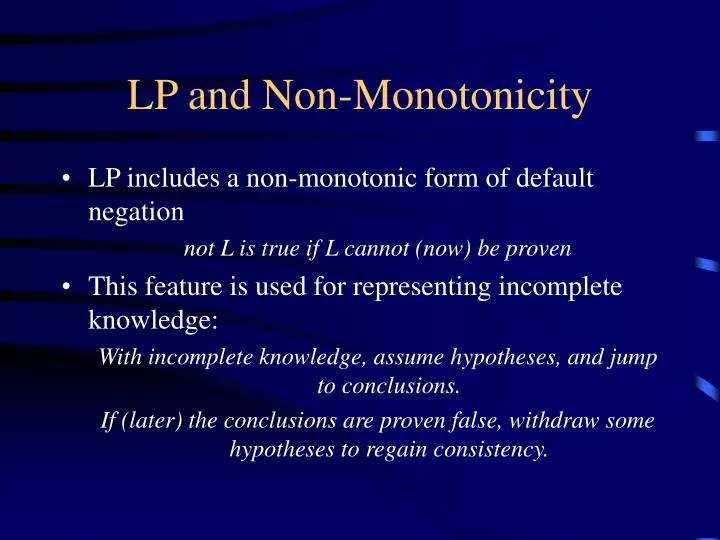
1. LP and Non-Monotonicity • LP includes a non-monotonic form of default negation not L is true if L cannot (now) be proven • This feature is used for representing incomplete knowledge: With incomplete knowledge, assume hypotheses, and jump to conclusions. If (later) the conclusions are proven false, withdraw some hypotheses to regain consistency.

2. Typical example • All birds fly. Penguins are an exception: flies(X)  bird(X), not ab(X). bird(a) . ab(X)  penguin(X). This program concludes flies(a), by assuming not ab(a). • If later we learn penguin(a): • Add: penguin(a). • Goes back on the assumption not ab(a). • No longer concludes flies(a).

3. LP representing a static world • The work on LP allows the (non-monotonic) addition of new knowledge. • But: • What we have seen so far does not consider this evolution of knowledge • LPs represent a static knowledge of a given world in a given situation. • The issues of how to add new information to a logic program wasn’t yet addressed.

4. Knowledge Evolution • Up to now we have not considered evolution of the knowledge • In real situations knowledge evolves by: • completing it with new information • changing it according to the changes in the world itself • Simply adding the new knowledge possibly leads to contradiction • In many cases a process for restoring consistency is desired

5. Revision and Updates • In real situations knowledge evolves by: • completing it with new information (Revision) • changing it according to the changes in the world itself (Updates) • These forms of evolution require a differentiated treatment. Example: • I know that I have a flight booked for London (either for Heathrow or for Gatwick). Revision: I learn that it is not for Heathrow • I conclude my flight is for Gatwick Update: I learn that flights for Heathrow were canceled • Either I have a flight for Gatwick or no flight at all

6. AGM Postulates for Revision For revising a logical theory T with a formula F, first modify T so that it does not derive ¬F, and then add F. The contraction of T by a formula F, T-(F), should obey: • T-(F) has the same language as T • Th(T-(F))  Th(T) • If T |≠ F then T-(F) = T • If |≠ F then T-(F) |≠ F • Th(T)  Th(T-(F)  {F}) • If |= F ↔ G then Th(T-(F)) = Th(T-(G)) • T-(F) ∩ T-(G)  T-(F  G) • If T-(F  G) |≠ F then T-(F  G)  T-(F)

7. Epistemic Entrenchment • The question in general theory revision is how to change a theory so that it obeys the postulates? • What formulas to remove and what formulas to keep? • In general this is done by defining preferences among formulas: some can and some cannot be removed. • Epistemic Entrenchment: some formulas are “more believed” than others. • This is quite complex in general theories. • In LP, there is a natural notion of “more believed”

8. The problem: A LP represents consistent incomplete knowledge; New factual information comes. How to incorporate the new information? The solution: Add the new facts to the program If the union is consistent this is the result Otherwise restore consistency to the union Logic Programs Revision • The new problem: • How to restore consistency to an inconsistent program?

9. Simple revision example (1) P: flies(X)  bird(X), not ab(X). bird(a) . ab(X)  penguin(X). • We learn penguin(a). • P  {penguin(a)} is consistent. Nothing more to be done. • We learn instead ¬flies(a). • P  {¬flies(a)} is inconsistent. What to do? • Since the inconsistency rests on the assumption not ab(a), remove that assumption (e.g. by adding the fact ab(a), or forcing it undefined with ab(a) u) obtaining a new program P’. If an assumption supports contradiction, then go back on that assumption.

10. Simple revision example (2) P: flies(X)  bird(X), not ab(X). bird(a) . ab(X)  penguin(X). If later we learn flies(a). P’  {flies(a)} is inconsistent. The contradiction does not depend on assumptions. Cannot remove contradiction! Some programs are non-revisable.

11. What to remove? • Which assumptions should be removed? normalWheelnot flatTyre, not brokenSpokes. flatTyreleakyValve. ¬normalWheelwobblyWheel. flatTyrepuncturedTube. wobblyWheel. • Contradiction can be removed by either dropping not flatTyre or not brokenSpokes • We’d like to delve deeper in the model and (instead of not flatTyre) either drop not leakyValve or not puncturedTube.

12. Revisables • Solution: • Define a set of revisables: normalWheelnot flatTyre, not brokenSpokes. flatTyreleakyValve. ¬normalWheelwobblyWheel. flatTyrepuncturedTube. wobblyWheel. Revisables = not {leakyValve, punctureTube, brokenSpokes} Revisions in this case are {not lv}, {not pt}, and {not bs}

13. Integrity Constraints • For convenience, instead of: ¬normalWheel  wobblyWheel we may use the denial:  normalWheel, wobblyWheel • ICs can be further generalized into: L1 …  Ln Ln+1 …  Lm where Lis are literals (possibly not L).

14. ICs and Contradiction • In an ELP with ICs, add for every atom A:  A, ¬A • A program P is contradictory iff P   where  is the paraconsistent derivation of SLX

15. Algorithm for 3-valued revision • Find all derivations for , collecting for each one the set of revisables supporting it. Each is a support set. • Compute the minimal hitting sets of the support sets. Each is a removal set. • A revision of P is obtained by adding {A u: A  R} where R is a removal set of P.

16. (Minimal Hitting Sets) • H is a hitting set of S = {S1,…Sn} iff • H ∩ S1≠ {} and … H ∩ Sn≠ {} • H is a minimal hitting set of S iff it is a hitting set of S and there is no other hitting set of S, H’, such that H’ Í H. • Example: • Let S = {{a,b},{b,c}} • Hitting sets are {a,b},{a,c},{b},{b,c},{a,b,c} • Minimal hitting sets are {b} and {a,c}.

17.  p q not a r not b not c not b Example Rev = not {a,b,c}   p, q p  not a. q  not b, r. r  not b. r  not c. {not a, not b} and {not a, not b, not c}. Support sets are: Removal sets are: {not a} and {not b}.

18. a=1 b0 g1 Simple diagnosis example inv(G,I,0)  node(I,1), not ab(G). inv(G,I,1)  node(I,0), not ab(G). node(b,V)  inv(g1,a,V). node(a,1). ¬node(b,0). %Fault model inv(G,I,0)  node(I,0), ab(G). inv(G,I,1)  node(I,1), ab(G). The only revision is: P U {ab(g1) u} It does not conclude node(b,1). • In diagnosis applications (when fault models are considered) 3-valued revision is not enough.

19. 2-valued Revision • In diagnosis one often wants the IC: ab(X) v not ab(X)  • With these ICs (that are not denials), 3-valued revision is not enough. • A two valued revision is obtained by adding facts for revisables, in order to remove contradiction. • For 2-valued revision the algorithm no longer works…

20.  a p not c b X not a not b X • P U {a} is contradictory (and unrevisable). • P U {b} is contradictory (though revisable). But: Example   p.  a.  b, not c. p  not a, not b. • In 2-valued revision: • some removals must be deleted; • the process must be iterated. The only support is {not a, not b}. Removals are {not a} and {not b}.

21. Algorithm for 2-valued revision • Let Revs={{}} • For every element R of Revs: • Add it to the program and compute removal sets. • Remove R from Revs • For each removal set RS: • Add R U not RS to Revs • Remove non-minimal sets from Revs • Repeat 2 and 3 until reaching a fixed point of Revs. The revisions are the elements of the final Revs.

22. Example of 2-valued revision   p.  a.  b, not c. p  not a, not b. Rev0 = {{}} Rev1 = {{a}, {b}} Rev2 = {{b}} Rev3 = {{b,c}} = Rev4 • Choose {}. Removal sets of P U {} are {not a} and {not b}. Add them to Rev. • Choose {a}. P U {a} has no removal sets. • Choose {b}. The removal set of P U {b} is {not c}. Add {b, c} to Rev. • Choose {b,c}. The removal set of P U {b,c} is {}. Add {b, c} to Rev. • The fixed point had been reached. P U {b,c} is the only revision.

23. Revision and Diagnosis • In model based diagnosis one has: • a program P with the model of a system (the correct and, possibly, incorrect behaviors) • a set of observations O inconsistent with P (or not explained by P). • The diagnoses of the system are the revisions of P  O. • This allows to mixed consistency and explanation (abduction) based diagnosis.

24. c1=0 1 0 g10 g22 c3=0 c2=0 1 g16 1 c6=0 g11 1 0 1 c7=0 g23 g19 Diagnosis Example

25. Diagnosis Program Observables obs(out(inpt0, c1), 0). obs(out(inpt0, c2), 0). obs(out(inpt0, c3), 0). obs(out(inpt0, c6), 0). obs(out(inpt0, c7), 0). obs(out(nand, g22), 0). obs(out(nand, g23), 1). Connections conn(in(nand, g10, 1), out(inpt0, c1)). conn(in(nand, g10, 2), out(inpt0, c3)). … conn(in(nand, g23, 1), out(nand, g16)). conn(in(nand, g23, 2), out(nand, g19)). Predicted and observed values cannot be different  obs(out(G, N), V1), val(out(G, N), V2), V1  V2. Value propagation val( in(T,N,Nr), V )  conn( in(T,N,Nr), out(T2,N2) ), val( out(T2,N2), V ). val( out(inpt0, N), V )  obs( out(inpt0, N), V ). Normal behavior val( out(nand,N), V ) not ab(N), val( in(nand,N,1), W1), val( in(nand,N,2), W2), nand_table(W1,W2,V). Abnormal behavior val( out(nand,N), V ) ab(N), val( in(nand,N,1), W1), val( in(nand,N,2), W2), and_table(W1,W2,V).

26. c1=0 1 1 1 0 0 0 0 g10 g22 c3=0 c2=0 0 1 1 g16 1 1 1 c6=0 g11 1 1 1 1 0 1 1 c7=0 g23 g19 Diagnosis Example , and {ab(g16),ab(g22)} , {ab(c19)} Revision are: {ab(g23)}

27. Revision and Debugging • Declarative debugging can be seen as diagnosis of a program. • The components are: • rule instances (that may be incorrect). • predicate instances (that may be uncovered) • The (partial) intended meaning can be added as ICs. • If the program with ICs is contradictory, revisions are the possible bugs.

28. Debugging Transformation • Add to the body of each possibly incorrect rule r(X) the literal not incorrect(r(X)). • For each possibly uncovered predicate p(X) add the rule: p(X)  uncovered(p(X)). • For each goal G that you don’t want to prove add:   G. • For each goal G that you want to prove add:   not G.

29. Debugging example WFM = {not a, b, not c} b should be false a ¬ not b b ¬ not c BUT a should be false! Add ¬ a Revisions now are: {inc(b ¬ not c), inc(a ¬ not b)} {unc(c ), inc(a ¬ not b)} a ¬ not b, not incorrect(a ¬ not b) b ¬ not c, not incorrect(b ¬ not c) a ¬ uncovered(a) b ¬ uncovered(b) c ¬ uncovered(c) ¬ b Revisables are incorrect/1 and uncovered/1 BUT c should be true! Add ¬ not c The only revision is: {unc(c ), inc(a ¬ not b)} Revision are: {incorrect(b ¬ not c)} {uncovered(c)}

30. Deduction, Abduction and Induction • In deductive reasoning one derives conclusions based on rules and facts • From the fact that Socrates is a man and the rule that all men are mortal, conclude that Socrates is mortal • In abductive reasoning given an observation and a set of rules, one assumes (or abduce) a justification explaining the observation • From the rule that all men are mortal and the observation that Socrates is mortal, assume that Socrates being a man is a possible justification • In inductive reasoning, given facts and observations induce rules that may synthesize the observations • From the fact that Socrates (and many others) are man, and the observation that all those are mortal induce that all men are mortal.

31. Deduction, Abduction and Induction • Deduction: an analytic process based on the application of general rules to particular cases, with inference of a result • Induction: synthetic reasoning which infers the rule from the case and the result • Abduction: synthetic reasoning which infers the (most likely) case given the rule and the result

32. Abduction in logic • Given a theory T associated with a set of assumptions Ab (abducibles), and an observation G (abductive query), D is an abductive explanation (or solution) for G iff: • D Ab • T D |= G • T D is consistent • Usually minimal abductive solutions are of special interest • For the notion of consistency, in general integrity constraints are also used (as in revision)

33. Abduction example wobbleWheelflatTyre. wobbleWheelbrokenSpokes. flatTyreleakyValve. flatTyrepuncturedTube. • It has been observed that wobblyWheel. • What are the abductive solutions for that, assuming that abducibles are brokenSpokes, leakyValve and puncturedTube?

34. Applications • In diagnosis: • Find explanations for the observed behaviour • Abducible are the normality (or abnormality) of components, and also fault modes • In view updates • Find extensional data changes that justify the intentional data change in the view • This can be further generalized for knowledge assimilation

35. Abduction as Nonmonotonic reasoning • If abductive explanations are understood as conclusions, the process of abduction is nonmonotonic • In fact, abduction may be used to encode various other forms of nonmonotonic logics • Vice-versa, other nonmonotonic logics may be used to perform abductive reasoning

36. Negation by Default as Abduction • Replace all not A by a new atom A* • Add for every A integrity constraints: A  A*   A, A* • L is true in a Stable Model iff there is an abductive solution for the query F • Negation by default is view as hypotheses that can be assumed consistently

37. Defaults as abduction • For each rule d: A : B C add the rule C ← d(B), A and the ICs ¬d(B) ¬ B ¬d(B) ¬C • Make all d(B) abducible

38. Abduction and Stable Models • Abduction can be “simulated” with Stable Models • For each abducible A, add to the program: A ← not ¬A ¬A ← not A • For getting abductive solutions for G just collect the abducibles that belong to stable models with G • I.e. compute stable models after also adding ← not G and then collect all abducible from each stable model

39. Abduction and Stable Models (cont) • The method suggested lacks means for capturing the relevance of abductions made for really proving the query • Literal in the abductive solution may be there because they “help” on proving the abductive query, or simply because they are needed for consistency independently of the query • Using a combination of WFS and Stable Models may help in this matter.

40. Abduction as Revision • For abductive queries: • Declare as revisable all the abducibles • If the abductive query is Q, add the IC:   not Q • The revision of the program are the abductive solutions of Q.