Download
1 / 89
960 likes | 1.34k Views
The DMAIC Lean Six Sigma Project and Team Tools Approach Analyze Phase (Part 2). Lean Six Sigma Black Belt Training! Analyze (Part 2) Agenda. Review Analyze Part 1 Inferential Statistics Hypothesis Testing P-values Discrete X / Continuous Y Statistical Tests

E N D
The DMAIC Lean Six Sigma Project and Team Tools Approach Analyze Phase(Part 2)
Lean Six Sigma Black Belt Training! Analyze (Part 2) Agenda Review Analyze Part 1 Inferential Statistics Hypothesis Testing P-values Discrete X / Continuous Y Statistical Tests Continuous X / Continuous Y Statistical Tests Discrete X / Discrete Y Statistical Tests Applications / Lessons Learned / Conclusions Next Steps
Six Sigma AnalyzeInferential Statistics (Identifying What’s Different (Xs) Statistically)
Introduction to Hypothesis Testing Are these samples from the same population? Sample 1 Sample 2 Mean=6.5 StDev=1 Mean=6.9 StDev=1.2
Intro. to Confidence Intervals (pg. 157) Brutal Facts Regarding Samples We know that the size of the sampling error is primarily based on the variation in the population and the size of the sample selected. Larger samples have a smaller margin or error, yet are more costly to obtain. As reality in practice dictates, one sample is usually selected and it usually is the minimum size required. Therefore, a method was needed to estimate a population parameter. This method resulted in the term Confidence Interval. 5
Intro. to Confidence Intervals (pg. 157) A statistic plus or minus a margin of error is called a confidence interval. A confidence interval is a range of values, calculated from a data set, that gives an assigned probability that the true value falls within that range. The confidence level is dependent on the range of the margin of error that is selected. Generally, the margin of error that is accepted is plus or minus 2 standard errors, resulting in a 95% confidence level. “We are 95% confident that the true average door-to-balloon time is between 60 and 100 minutes.”
50 Assume we have a population of N size that is not normally distributed. We draw 100 random samples and plot the averages of each sample. We get a normal distribution with a mean of 50 and n=100.
68% 95% 50 +2 SE +1 SE -1 SE -2 SE The mean of our sampled distribution is 50. How confident are we of where the population mean lies? Similar to standard deviation, we know that 68% of the sample distribution lies within 1 standard error and 95% within 2 standard errors.
SE = 95% σ √ n 50 +2 SE +1 SE -1 SE -2 SE • The mean of our sample • distribution is 50. • We are 95% confident that • the true mean of the • population lies between 44 • and 56. • Our margin of error is +/- 6. Let’s assume we want to be 95% confident of where the true mean of the population lies We can be 95% confident that the true mean lies within +/- 2SE In this case, let’s assume that SE=3, so 2 x SE = 6.
Central Limit Theorem/ Margin of Error/ Confidence Intervals Why Use it? Why is this important? Six Sigma practitioners use the sample data and apply normal theory for making inferences about population parameters irrespective of the actual form of the parent population. Many statistical tests are founded on the principle that we do not need to know the original distribution. Means and proportions will always be “normal” if n is big enough. Practically, we use the central limit theorem to help us estimate the true average, and calculate the likelihood of observing certain events. Considering time and resources, we need to have a measure of confidence around our sample statistics. None of this is applicable if your data is Unreliable or BIASED!!!!
Data-Driven Problem Solving:Hypothesis Testing Two fundamental questions must be adequately answered in order to be able to adequately perform hypothesis testing: What type of data is available (and reliable)? What question are you asking (what do you need to understand)?
Introduction to Hypothesis Testing (pg. 156) Hypothesis testing is basically the process of using statistical analysis to determine if the observed differences between two or more sets of data are due to random chance variation, or due to true differences in the underlying populations. Generally, Hypothesis Testing tells us whether or not sets of data are truly different with a certain level of confidence.
Introduction to Hypothesis Testing Are these samples from the same population? Sample 1 Sample 2 Mean=6.5 StDev=1 Mean=6.9 StDev=1.2
The Six Sigma Approach Statistical Problem – Defining the problem in statistical terms Practical Problem – An unacceptable variation or gap in quality Statistical Solution – Using data and statistics to understand the cause of the problem Practical Solution – addresses the verified root causes Practical Problem – Lab specimens are mislabeled too often; leads to incorrect diagnosis and treatment Statistical Problem – Specimens are mislabeled 8 out of 10,000 collected Practical Solution – Redesign of the process of labeling and transporting specimens leads to dramatic reduction in errors Statistical Solution – ~85% of mislabeled specimens come from the ED Six Sigma applies many tools, including statistical tools to practical problems. The key is data-driven decision making.
Introduction to Hypothesis Testing Hypothesis Testing allows us to answer a practical question - Is there a true difference between ___ and ___ ? Practically, Hypothesis Testing uses relatively small sample sizes to answer questions about the population. There is always a chance that the samples we have collected are not truly representative of the population. Thus, we may obtain a wrong conclusion about the population(s) being studied.
Introduction to Hypothesis Testing:Testing Terms and Concepts Statistically, we “ask and answer questions” using stated hypotheses that are tested at some level of confidence. Thenull hypothesis (Ho) is a statement being tested to determine whether or not it is true (the assumption that there is no difference). Thealternative hypothesis (Ha) is a statement that represents reality if there is enough evidence to reject the stated null (Ho)… i.e. the null hypothesis is false.
Introduction to Hypothesis Testing Example: Is the average Length of Stay for a total knee replacement different for Hospital A vs. Hospital B? Common Language: Ho: There is no difference in average length of stay between facilities. Ha: There is a difference in average length of stay between facilities. Statistical Language: Ho: mAlos = mBlos Ha: mAlos≠mBlos
Introduction to Hypothesis Testing:Type I and Type II Errors (Risk) As stated earlier, there is the risk of arriving at a wrong conclusion about the hypothesis we are testing. The two types of error that can occur with hypothesis testing are called Type I and Type II. The associated risks are called Alpha and Beta risks. A Type I (Alpha) error is concluding there is a difference when there really isn’t one. - Rejecting the null when you should not! A Type II (Beta) error is concluding there is not a difference when there really is one. - Do not reject the null when you should!
Type I and Type II errors,Confidence, Power, and p-values Correct Type I Error (a risk) Type II Error (b risk) Correct Conclusion Drawn You conclude there IS a difference when there really isn’t Do not reject H0 Reject H0 H0 is true The True Statement H0 is false You conclude there is NO difference when there really is
Type I and Type II errors in the Justice System Innocent person acquitted Innocent person convicted Guilty person acquitted Guilty person convicted Verdict Guilty Acquittal Did not commit crime True State Committed crime
Result MatrixHo: No difference between the accused and an innocent person The Truth The Truth
Introduction to p-value The p-value measures the probability of observing a certain amount of difference if the null hypothesis is true. In comparing the average length of stay (ALOS) at Hospitals A and B, p-value measures the likelihood of observing a difference in ALOS if the null hypothesis is true. If the p-value is large, then both averages probably came from the same population (i.e. there is no difference between ALOS at Hospital A and B). If the p-value is small, then it is unlikely both averages came from the same population (i.e. there is a difference between ALOS at Hospital A and B).
mean 40 40 50 P-Value (pg. 160)What’s the probability of getting a value of “40”? mean 50
Setting the Alpha threshold • Alpha (a) is the level of risk you are willing to accept of making a Type I error (i.e. rejecting the null when the null is true). • Traditionally, alpha (a) is set at 0.05, which means you are willing to accept a 5% chance of making a Type I error (i.e. rejecting the null when the null is true).
P-Value mean Fail to reject Fail to reject a region (reject) a region (reject) The critical value at which the null hypothesis is rejected. “If p is low, Ho must go” (usually at or below 0.05)
Hypothesis Testing – Basic Steps(see also pg 156-160) State the practical problem State the null hypothesis State the alternate hypothesis Test the assumptions of the data Determine appropriate alpha (a) decision value Calculate the appropriate test statistic and calculate p-value If calculated p-value < a, then reject Ho; if p-value > a then fail to reject Ho Formulate the statistical conclusion into a practical solution
Statistical Testing – Basic Steps What theory or potential cause is presented or proposed? Given the theory or potential cause in front of you, What is the question you are trying to answer? Do you have data directly related to and describing the question you are asking? What type of data do you have? If you do not have data, can you collect the appropriate data (reasonably and appropriately)? If no data exists relating to the theory being considered, or if it will be very costly to obtain, re-visit the magnitude and urgency of testing this particular theory. Proceed with data collection and sorting/grouping as needed. State the question as a null hypothesis (There is no difference…) State the alternate hypothesis Test the assumptions of the data as needed (normality, quantity, variances, etc.) Determine appropriate alpha (a) decision value (.05, etc.) Chose and calculate the appropriate test statistic (determined by the data you have and the question you are asking) and the associated p-value If calculated p-value < a, then reject Ho; if p-value > a then fail to reject Ho Formulate the statistical conclusion into a practical solution (answer to question)
Remember? - Data-Driven Problem Solving:Hypothesis Testing Two fundamental questions must be adequately answered in order to be able to adequately perform hypothesis testing: What type of data is available (and reliable)? What question are you asking (what do you need to understand)?
What Type of Data to Analyze: • Discrete X / Continuous Y • Continuous X / Continuous Y • Discrete X / Discrete Y
Data-Driven Analysis:Discrete X / Continuous Y • Descriptive Statistics: mean, median, variance, standard deviation • Graphical display: box plots, error bars, run charts • Potential Questions: Is there a difference in means, medians, variances
Variance Testing Distribution Normal Non-normal or unknown Sample
Test for Equal Variances Stat>Basic Statistics>2 Variances
Test for Equal Variances Test for Equal Variances: Quality versus Region 95% Bonferroni confidence intervals for standard deviations Region N Lower StDev Upper 1 116 2.13011 2.46845 2.92567 2 67 2.03534 2.46264 3.09934 3 100 2.58684 3.02983 3.64282 Bartlett's Test (Normal Distribution) Test statistic = 5.58, p-value = 0.061 Levene's Test (Any Continuous Distribution) Test statistic = 6.24, p-value = 0.002 Stat>Basic Statistics>2 Variances
Test for Equal Variances Stat>Basic Statistics>2 Variances
Hypothesis Testing:Discrete X / Continuous Y For : 1 Sample t-test (See page 162 in The Lean Six Sigma Pocket Toolbook) Ho:m equal to a target or known value Ha:m is not equal to a target or known value Statistical Test: One sample t-test Test Statistic: T-value – based on the area under the curve of an unknown or non-normal distribution
Hypothesis Testing:Discrete X / Continuous Y For : 2 Sample t-test (See page 182 in The Lean Six Sigma Pocket Toolbook) Ho:m1 = m2 Ha:m1≠m2 Statistical Test: 2 Sample t-test Test Statistic: T-value – based on the area under the curve of an unknown or non-normal distribution
Analyze Tools:Discrete X / Continuous Y See page 110 in The Lean Six Sigma Pocket Toolbook 3rd Quartile line Median line 1st Quartile line • Graphical display: Box plots • The box shows the range of data values comprising the 2nd and 3rd quartiles of the data – the “middle” 50% of the data
Analyze Tools: Box Plots 25% 25% 25% 25% 14 1st Quartile Outlier * Extends to largest value within 3Q+1.5 x IQR The Inter Quartile Range (IQR) is the range encompassed by the 2nd Quartile and 3rd Quartile… 6-4=2 3rd Quartile 2nd Quartile 5 Median Median= 4.5 2nd Quartile Extends to smallest value within 2Q-1.5 x IQR 3rd Quartile 0 4th Quartile There are 24 entries in this table
Data-Driven Analysis:Continuous X / Continuous Y • Descriptive Statistics: correlation • Graphical Display: scatter plot, run charts • See 165-175 in The Lean Six Sigma Toolbook
Analyze Tools:Continuous X / Continuous Y • Correlation indicates whether there is a relationship between the values of two measurements • Positive correlation: higher values in X are associated with higher values in Y • Negative correlation: higher values in X are associated with lower values in Y. • Correlation does NOT imply cause-and-effect! • Correlation could be coincidence • Both variables could be influenced by some lurking variable
Hypothesis TestingCorrelation Statistics • Regression analysis generates correlation coefficients to indicate the strength and nature of the relationship • Pearson correlation coefficient (r): the strength and direction of the relationship • Between 1 and -1 • r2:percent of variation in Y that is attributable to X • Between 0 and 1
Hypothesis Testing:Continuous X/Continuous Y For : Regression and Correlation (pg. 168) Ho: The slope of the line is equal to zero b1 = 0 Ha: The slope of the line does not equal zero b1≠ 0 Statistical Test: Regression Test Statistic: F ratio – a measure of actual to expected variation in the sample
Correlation Example Correlations: Clarity, Quality Pearson correlation of Clarity and Quality = 0.075 P-Value = 0.208 Stat>Basic Statistics>Correlation
Pearson’s r Rules of Thumb • Strength and direction of relationship between x and Y • 0 to .20: no or negligible correlation. • .20 to .40: low degree of correlation. • .40 to .60: moderate degree of correlation. • .60 to .80: marked degree of correlation. • .80 to 1.00: high correlation.
Regression Example Regression Analysis: Quality versus Clarity The regression equation is Quality = 11.7 + 1.02 Clarity Predictor Coef SE Coef T P Constant 11.6524 0.7253 16.06 0.000 Clarity 1.0234 0.8118 1.26 0.208 S = 2.82408 R-Sq = 0.6% R-Sq(adj) = 0.2% Analysis of Variance Source DF SS MS F P Regression 1 12.676 12.676 1.59 0.208 Residual Error 281 2241.094 7.975 Total 282 2253.770 Stat>Regression>Regression…
Regression Example 2 Regression Analysis: Quality versus Clarity The regression equation is Quality = 11.65 + 1.023 Clarity S = 2.82408 R-Sq = 0.6% R-Sq(adj) = 0.2% Analysis of Variance Source DF SS MS F P Regression 1 12.68 12.6757 1.59 0.208 Error 281 2241.09 7.9754 Total 282 2253.77 Stat>Regression>Fitted Line Plot… Analyze - Continuous X / Continuous Y